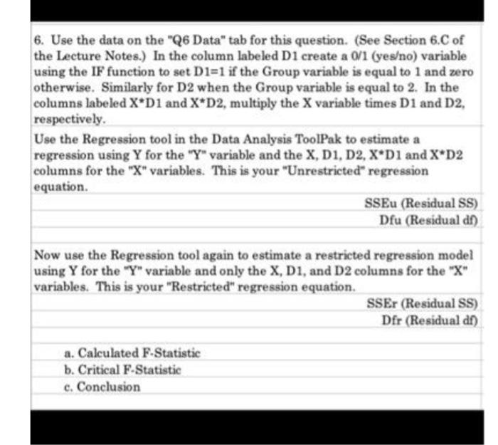
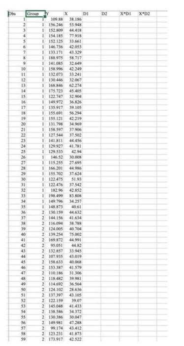
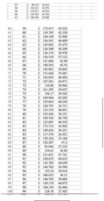
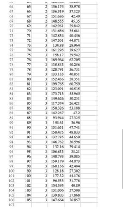
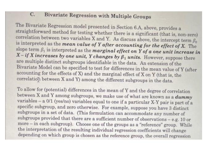6. Use the data on the "Q6 Data" tab for this question. (See Section 6.C of the Lecture Notes.) In the column labeled D1 create a 0/1 (yeso) variable using the IF function to set D1=1 if the Group variable is equal to 1 and zero otherwise. Similarly for D2 when the Group variable is equal to 2 . In the columns labeled XD1 and XD2, multiply the X variable times D1 and D2, respectively. Use the Regression tool in the Data Analysis ToolPak to estimate a regression using Y for the " Y" variable and the X,D1,D2,XD1 and XD2 columns for the "X" variables. This is your "Unrestricted" regression equation. SSEu(ResidualSS)Dfu(Residualdf) Now use the Regression tool again to estimate a restricted regression model using Y for the "Y" variable and only the X, D1, and D2 columns for the "X" variables. This is your "Restricted" regression equation. SSEr(ResidualSS)Dfr(Residualdf) a. Calculated F.Statistic b. Critical F-Statistic c. Conclusion \begin{tabular}{|r|r|r|r|} \hline 51 & 2 & 95.174 & 41.412 \\ \hline 58 & 2 & 121.211 & 41.573 \\ \hline 59 & 2 & 173.917 & 42.522 \\ \hline 60 & 2 & 154.783 & 42334 \\ \hline 61 & 2 & 144.149 & 13504 \\ \hline \end{tabular} The Bivariate Regression model presented in Section 6.A, above, provides a straightforward method for testing whether there is a significant (that is, non-zero) correlation between two variables X and Y. As discuss above, the intercept term 0 is interpreted as the mean value of Y after accounting for the effect of X. The slope term 1 is interpreted as the marginal effect on Y of a one unit increase in X - if X increases by one unit, Y changes by 1 units. However, suppose there are multiple distinct subgroups identifiable in the data. An extension of the Bivariate Model can be specified to test for differences in the mean value of Y (after accounting for the effects of X ) and the marginal effect of X on Y (that is, the correlation between X and Y ) among the different subgroups in the data. To allow for (potential) differences in the mean of Y and the degree of correlation between X and Y among subgroups, we make use of what are known as a dummy variables - a 0/1 (yeso) variables equal to one if a particular X-Y pair is part of a specific subgroup, and zero otherwise. For example, suppose you have 3 distinct subgroups in a set of data. (This formulation can accommodate any number of subgroups provided that there are a sufficient number of observations - e.g. 10 or more - in each subgroup). Choose one of the groups as a "reference" group. While the interpretation of the resulting individual regression coefficients will change depending on which group is chosen as the reference group, the overall regression 6. Use the data on the "Q6 Data" tab for this question. (See Section 6.C of the Lecture Notes.) In the column labeled D1 create a 0/1 (yeso) variable using the IF function to set D1=1 if the Group variable is equal to 1 and zero otherwise. Similarly for D2 when the Group variable is equal to 2 . In the columns labeled XD1 and XD2, multiply the X variable times D1 and D2, respectively. Use the Regression tool in the Data Analysis ToolPak to estimate a regression using Y for the " Y" variable and the X,D1,D2,XD1 and XD2 columns for the "X" variables. This is your "Unrestricted" regression equation. SSEu(ResidualSS)Dfu(Residualdf) Now use the Regression tool again to estimate a restricted regression model using Y for the "Y" variable and only the X, D1, and D2 columns for the "X" variables. This is your "Restricted" regression equation. SSEr(ResidualSS)Dfr(Residualdf) a. Calculated F.Statistic b. Critical F-Statistic c. Conclusion \begin{tabular}{|r|r|r|r|} \hline 51 & 2 & 95.174 & 41.412 \\ \hline 58 & 2 & 121.211 & 41.573 \\ \hline 59 & 2 & 173.917 & 42.522 \\ \hline 60 & 2 & 154.783 & 42334 \\ \hline 61 & 2 & 144.149 & 13504 \\ \hline \end{tabular} The Bivariate Regression model presented in Section 6.A, above, provides a straightforward method for testing whether there is a significant (that is, non-zero) correlation between two variables X and Y. As discuss above, the intercept term 0 is interpreted as the mean value of Y after accounting for the effect of X. The slope term 1 is interpreted as the marginal effect on Y of a one unit increase in X - if X increases by one unit, Y changes by 1 units. However, suppose there are multiple distinct subgroups identifiable in the data. An extension of the Bivariate Model can be specified to test for differences in the mean value of Y (after accounting for the effects of X ) and the marginal effect of X on Y (that is, the correlation between X and Y ) among the different subgroups in the data. To allow for (potential) differences in the mean of Y and the degree of correlation between X and Y among subgroups, we make use of what are known as a dummy variables - a 0/1 (yeso) variables equal to one if a particular X-Y pair is part of a specific subgroup, and zero otherwise. For example, suppose you have 3 distinct subgroups in a set of data. (This formulation can accommodate any number of subgroups provided that there are a sufficient number of observations - e.g. 10 or more - in each subgroup). Choose one of the groups as a "reference" group. While the interpretation of the resulting individual regression coefficients will change depending on which group is chosen as the reference group, the overall regression