6.2. Using Output 6.2: (a) How does combining (aggregating) mother's education and father's education and eliminating competence and pleasure scales change the results from those in Output 6.1? (b) Why did we aggregate mother's education and father's education? (c) Why did we eliminate the competence and pleasure scales?

The SPSS Outputs from the textbook are attached.

Leech, N. L., Barrett, K. C., & Morgan, G. A. (2014). IBM SPSS for Intermediate Statistics (5th ed.). Taylor & Francis. https://reader.yuzu.com/books/9781136334931

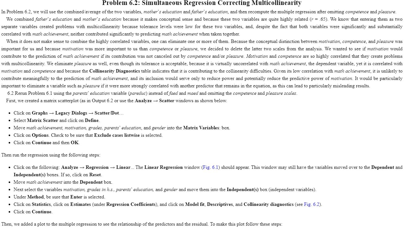
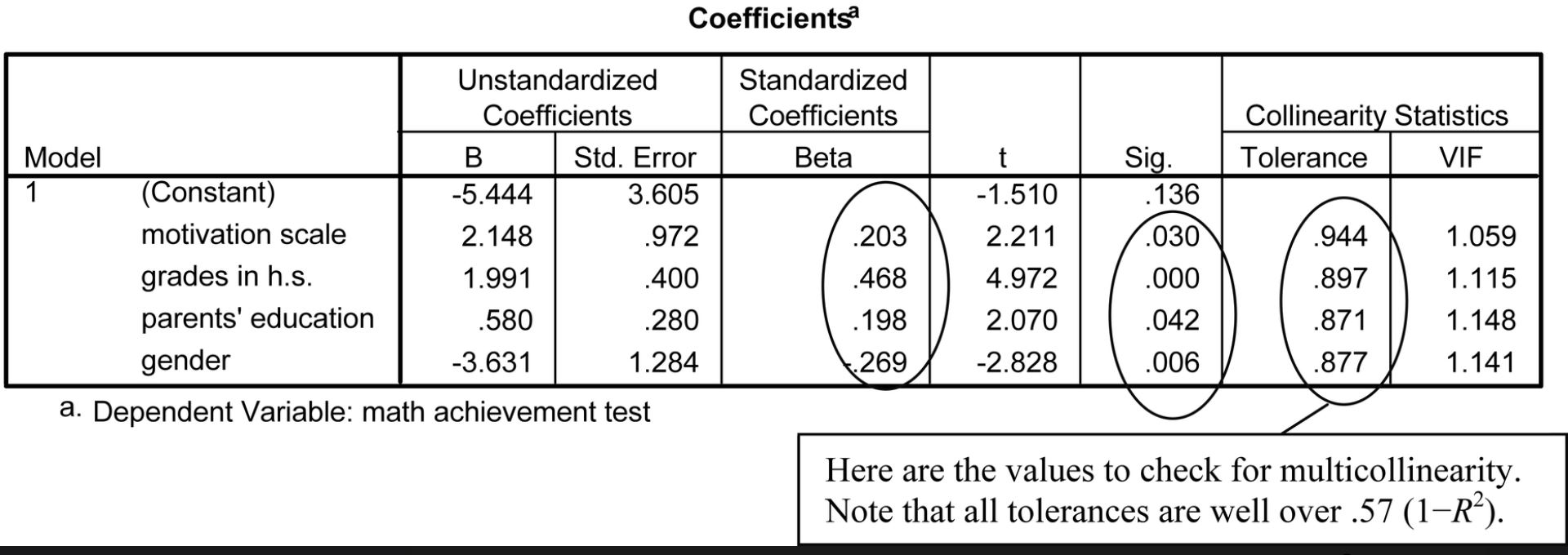
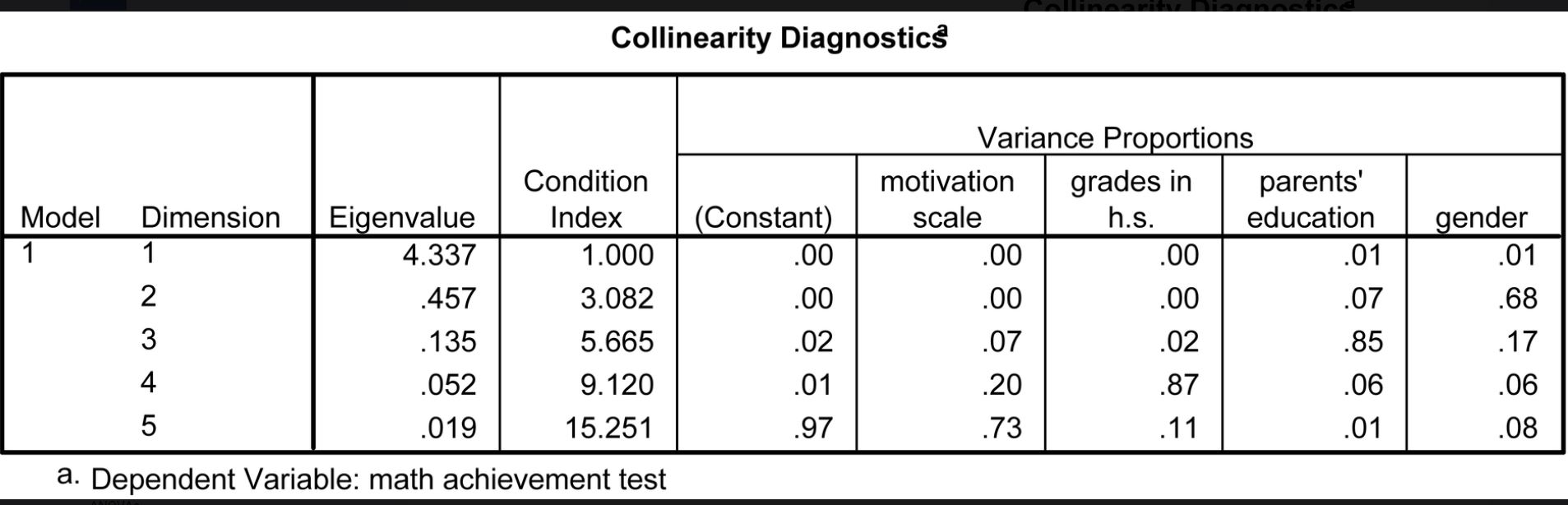
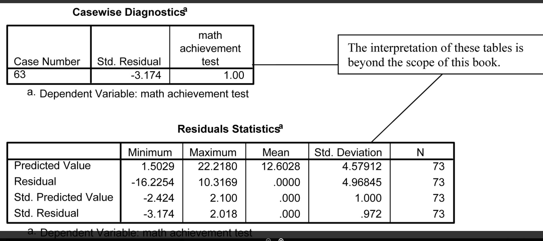
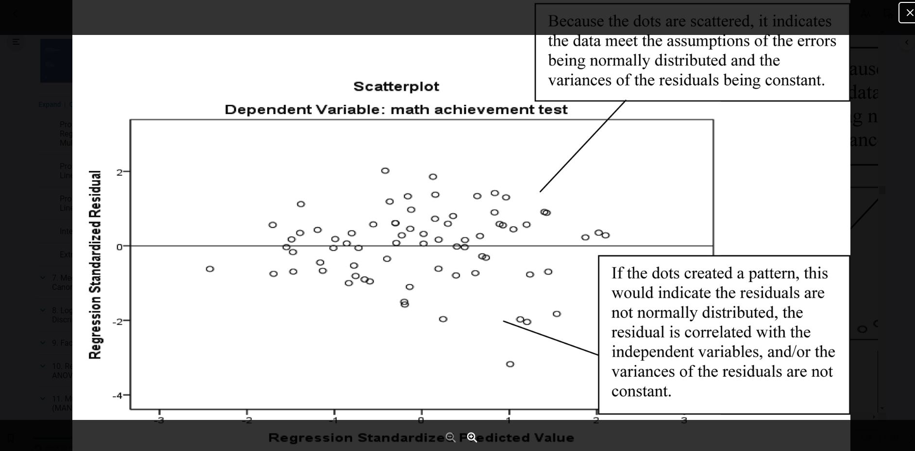
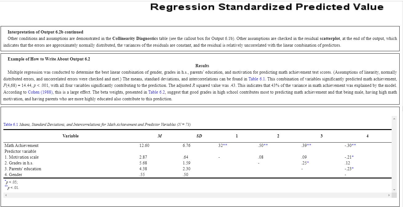
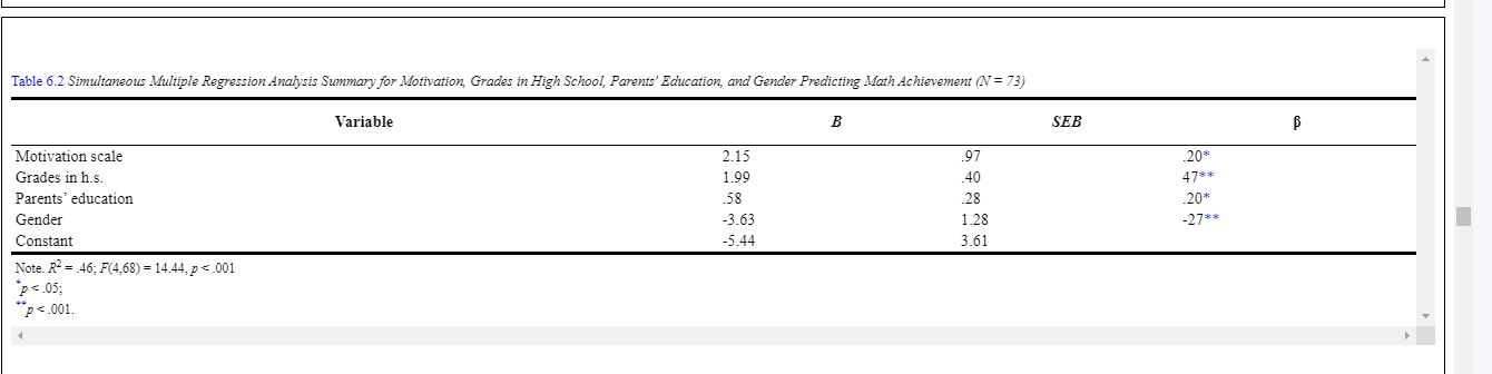
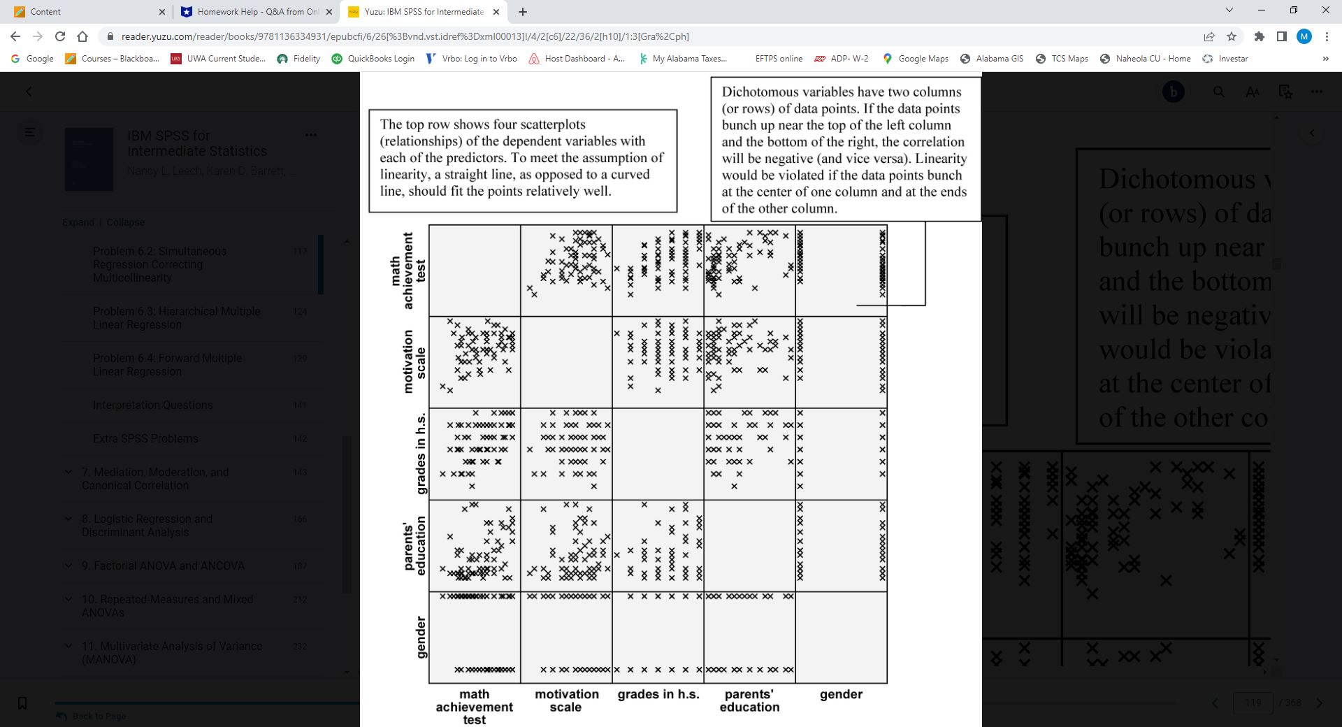
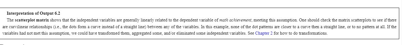
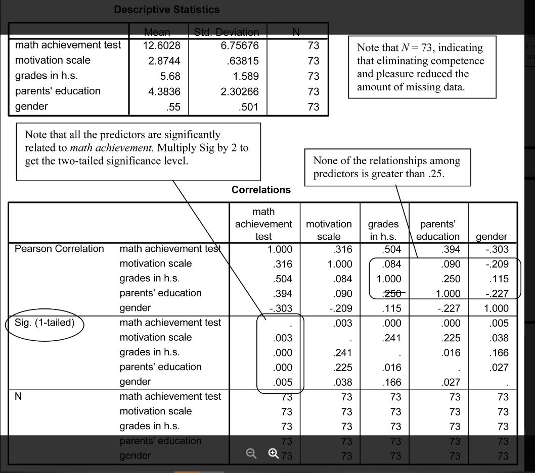
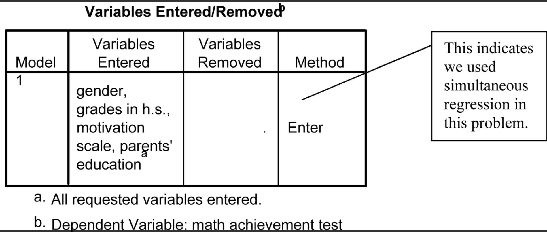
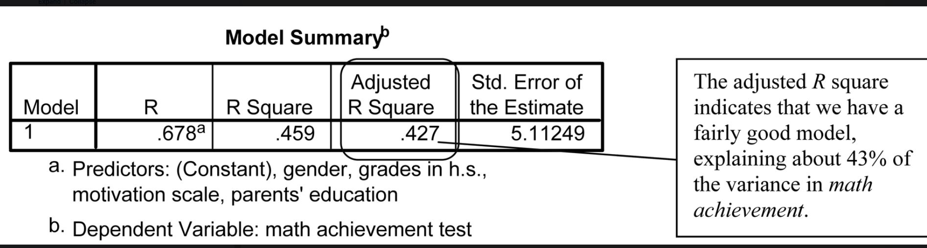
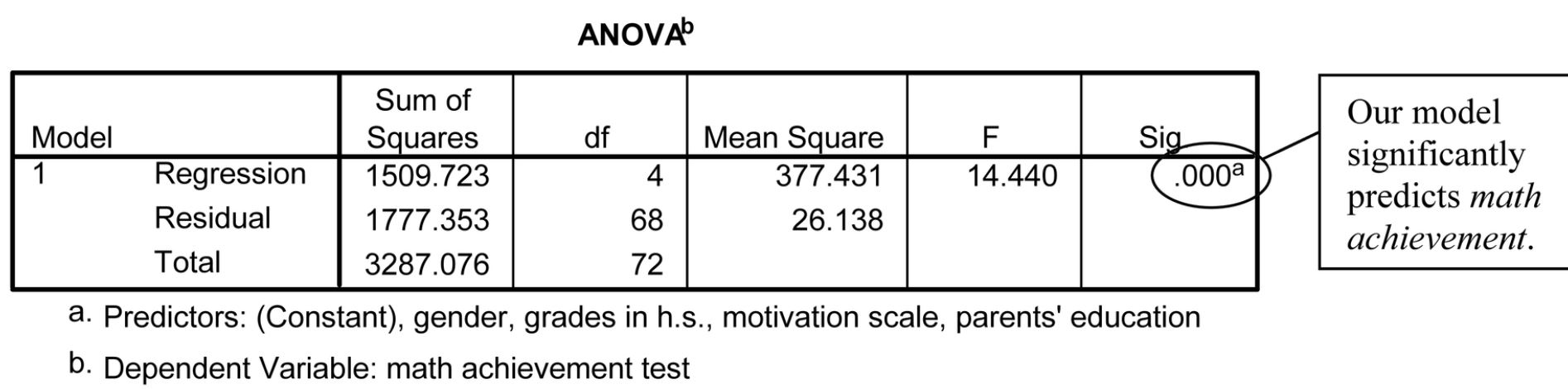
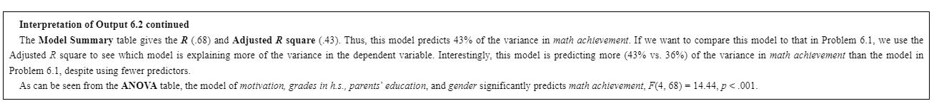
Problem 6.2: Simultaneous Regression Correcting Multicoilineal'iw In Problem 6.2. we Will use the combined'average ofthe two variables. mother's education andfothefs education. and then recompute the multiple regression aer omitting competence andpfeasure we combined father's education and mother's education because it makes conceptual sense and because these two variables are quite highly related (r = 65). We lcnow that entering them as two separate variables created problems With rnulticollinearitr because tolerance levels were low for these two variables. and. despite the fact that both variables were Significantly arid substantially correlated with math achiei-emeut. neither contributed significantly to predicting math achievement when taken together. \"lien it does not make sense to combine the highly correlated variables. one can eliminate one or more of them. Because the conceptual distinction between motivation. competence. and pleasure was important for us and because motivation was more important to us than competence or pleasure. we decided to delete the latter two scales from the analysis. We wanted to see if motivation would contribute to the prediction of math achievement if its contribution was not canceled out by competence and'or pleasure. limitation and competence are so highly correlated that they create problems with multicollinearity. We eliminate pleasure as well. even though its tolerance is acceptable. because it is virtually uncorrelated \"'lth math achievement. the dependent variable. yet it is correlated with motivation and competence and because the Collinearity Diagnostics table indicates that it is contributing to the collinearity diicul'ties. Given its low correlation with mark achievement. it is unlikely to contribute meaningfully to the prediction of math achiet emem'. and its inclusion would serve only to reduce power and potentially reduce the predictive power of motivation. It would be particularly important to eliminate avariahle such as pleasure if it were more strongly correlated with another predictor that remains in the equation. as this can lead to particularly misleading results 6.2 Ream Problem 6.1 using the parents education variable (pareo'uc) instead offaea' and maed and omitting the competence andpi'easure scales. First. we created a matrix scatterplot {as in Output 6.2 or use the Analyze > Scatter windows as shown below. - Click on Graphs a Legacy Dialogs ~ Station-\"Dot... - Select hiatrisr Scatter and click on Define I Move mat}: achievement. motivation grades. parents" education. and gender into the )Iatris Variables: box. 0 Click on Options. Check to be sure that Exclude cases listwise is selected. 0 Click on Continue and then OK Then run the regression using the following steps: 0 Click on the following: Analyze > Regression ' Linear... The Linear Regression window (Fig. 6.1) should appear. This. window may still have the variables moved over to the Dependent and Independent(s) boxes. If so. click on. Reset. - Move mat}: achievement mto the Dependent box. 0 Next select the variables motivation, grades or .5152. parents? education, and gender and move them into the Independens) box (independent variables) I Under )Iethod. be sure that Enter is selected. 0 Click on Statistics. click on Estimates (under Regression Coefficients). and click on Model fit. Descriptives. and Collinearity diagnostics (see Fig. 6.2). 0 Click on Continue. Then. we added a plot to the multiple regression to see the relationship ofthe predictors and the residual. To make this plot follow these steps: \fCasewise Diagnostics\" math achievement The interpretation of these tables is Case Number Std. Residual test beyond the scope of this book. 3-174 a. Dependent Variable: math achievement test Residuals Statistics3 ___'_3 Predicted Value 1 5029 22. 2180 12. 6028 4. 57912 Residual 16.2254 10.3169 .0000 4.96845 Std. Predicted Value -2.424 2.100 .000 1.000 Std. Residual -3.174 2.018 .000 .972 Interpretation of Output 6.2 The scarterplot matrix shows that the Independent variables are generally linearly related to the dependent variable of mark achievement, meeting this assumption. One should check the matrix scaerplots to see if there are curvilinear relationships (t.e._. the dots form a curve instead ofa straight line] between any ofthe variables. In this example. none ofthe dot patterns are closer to a curve then a straight line: or to no pattern at all. If the variables had not met this assumption we could have transformed them. aggregated some and or elimtnated some independent \\'ariahies. See Chapter 2 for hair to do transformations. \fInterpretation of Output 6.2 continued The Descriptive Table show that '.'.'.ll'.h this new set of variables we now have F3 students included. Note. that 4 more students no'n' have no missing data. which is good. In some samples one or a few t'asiahles may have a lot ofmissmg data= which is another reason that you might want to consider excluding them from your multiple regression or other multivariate statistics. The Correlation table shows that all predictors are significantly related to math achievement There are only low to moderate relationships among the four predictor variables. This is good because it suggests that collinearitt' is not high, a condition of multiple regression. \fInterpretation of Output 6.2 continued The Model Summary table gives the R (.683 and Adjusted .32 square [.43). Thus. this model predicts 43% of the variance in math achievement Ifu'e want to compare this model to that in Problem 6.1, we use the Adjusted R square to see which model is explaining more of the :'atiance in the dependent variable Iu'lerestmgljc= this model is predicting more (413% is 36%} of the variance in math achievement than the model in Problem 6.1 despiie usmg fewer predictors. As can. be seen from the ANOYA table. the model of math c2150; grade: i?! M, pareirrj' educarson. and gender significantly predicts mar}: achievement. F(4_. 68) = 14.44,;