Answered step by step
Verified Expert Solution
Question
1 Approved Answer
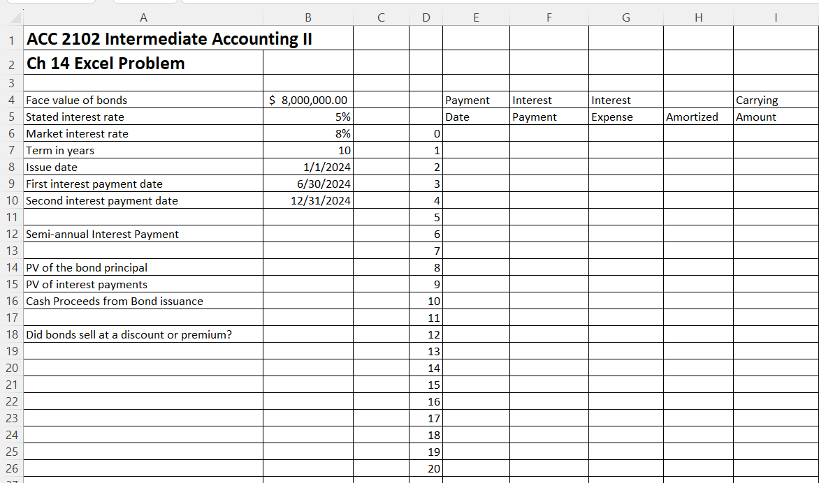
$8,000,000 is in B4 5% is B5 8% is B6 10 is B7 1/1/2024 is B8 6/30/2024 is B9 12/31/2024 is B10 0 starts in


$8,000,000 is in B4 5% is B5 8% is B6 10 is B7 1/1/2024 is B8 6/30/2024 is B9 12/31/2024 is B10
0 starts in column D6 and 20 ends in D26
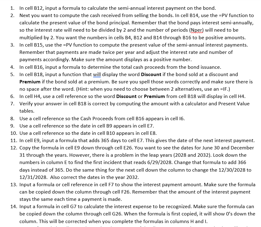
15. Input a formula in cell H7 to determine the amount of the discount or premium amortized. It will make the next formula easier if the amount of discount amortized is a positive number and the amount of premium amortized is a negative number. Copy the formula down through cell H26. 16. Input a formula in cell 17 to compute the new carrying value of the bonds and copy it down through cell I26. The amount in cell I26 should be equal to the face value of the bonds if your formulas are correct. 1. In cell B12, input a formula to calculate the semi-annual interest payment on the bond. 2. Next you want to compute the cash received from selling the bonds. In cell B14, use the =PV function to calculate the present value of the bond principal. Remember that the bond pays interest semi-annually, so the interest rate will need to be divided by 2 and the number of periods (Nper) will need to be multiplied by 2. You want the numbers in cells B4, B12 and B14 through B16 to be positive amounts. 3. In cell B15, use the =PV function to compute the present value of the semi-annual interest payments. Remember that payments are made twice per year and adjust the interest rate and number of payments accordingly. Make sure the amount displays as a positive number. 4. In cell B16, input a formula to determine the total cash proceeds from the bond issuance. 5. In cell B18, input a function that will display the word Discount if the bond sold at a discount and Premium if the bond sold at a premium. Be sure you spell those words correctly and make sure there is no space after the word. (Hint: when you need to choose between 2 alternatives, use an =IF.) 6. In cell H4, use a cell reference so the word Discount or Premium from cell B18 will display in cell H4. 7. Verify your answer in cell B18 is correct by computing the amount with a calculator and Present Value tables. 8. Use a cell reference so the Cash Proceeds from cell B16 appears in cell I6. 9. Use a cell reference so the date in cell B9 appears in cell E7. 10. Use a cell reference so the date in cell B10 appears in cell E8. 11. In cell E9, input a formula that adds 365 days to cell E7. This gives the date of the next interest payment. 12. Copy the formula in cell E9 down through cell E26. You want to see the dates for June 30 and December 31 through the years. However, there is a problem in the leap years (2028 and 2032). Look down the numbers in column E to find the first incident that reads 6/29/2028. Change that formula to add 366 days instead of 365 . Do the same thing for the next cell down the column to change the 12/30/2028 to 12/31/2028. Also correct the dates in the year 2032. 13. Input a formula or cell reference in cell F7 to show the interest payment amount. Make sure the formula can be copied down the column through cell F26. Remember that the amount of the interest payment stays the same each time a payment is made. 14. Input a formula in cell G7 to calculate the interest expense to be recognized. Make sure the formula can be copied down the column through cell G26. When the formula is first copied, it will show 0 's down the column. This will be corrected when you complete the formulas in columns H and I. 15. Input a formula in cell H7 to determine the amount of the discount or premium amortized. It will make the next formula easier if the amount of discount amortized is a positive number and the amount of premium amortized is a negative number. Copy the formula down through cell H26. 16. Input a formula in cell 17 to compute the new carrying value of the bonds and copy it down through cell I26. The amount in cell I26 should be equal to the face value of the bonds if your formulas are correct. 1. In cell B12, input a formula to calculate the semi-annual interest payment on the bond. 2. Next you want to compute the cash received from selling the bonds. In cell B14, use the =PV function to calculate the present value of the bond principal. Remember that the bond pays interest semi-annually, so the interest rate will need to be divided by 2 and the number of periods (Nper) will need to be multiplied by 2. You want the numbers in cells B4, B12 and B14 through B16 to be positive amounts. 3. In cell B15, use the =PV function to compute the present value of the semi-annual interest payments. Remember that payments are made twice per year and adjust the interest rate and number of payments accordingly. Make sure the amount displays as a positive number. 4. In cell B16, input a formula to determine the total cash proceeds from the bond issuance. 5. In cell B18, input a function that will display the word Discount if the bond sold at a discount and Premium if the bond sold at a premium. Be sure you spell those words correctly and make sure there is no space after the word. (Hint: when you need to choose between 2 alternatives, use an =IF.) 6. In cell H4, use a cell reference so the word Discount or Premium from cell B18 will display in cell H4. 7. Verify your answer in cell B18 is correct by computing the amount with a calculator and Present Value tables. 8. Use a cell reference so the Cash Proceeds from cell B16 appears in cell I6. 9. Use a cell reference so the date in cell B9 appears in cell E7. 10. Use a cell reference so the date in cell B10 appears in cell E8. 11. In cell E9, input a formula that adds 365 days to cell E7. This gives the date of the next interest payment. 12. Copy the formula in cell E9 down through cell E26. You want to see the dates for June 30 and December 31 through the years. However, there is a problem in the leap years (2028 and 2032). Look down the numbers in column E to find the first incident that reads 6/29/2028. Change that formula to add 366 days instead of 365 . Do the same thing for the next cell down the column to change the 12/30/2028 to 12/31/2028. Also correct the dates in the year 2032. 13. Input a formula or cell reference in cell F7 to show the interest payment amount. Make sure the formula can be copied down the column through cell F26. Remember that the amount of the interest payment stays the same each time a payment is made. 14. Input a formula in cell G7 to calculate the interest expense to be recognized. Make sure the formula can be copied down the column through cell G26. When the formula is first copied, it will show 0 's down the column. This will be corrected when you complete the formulas in columns H andStep by Step Solution
There are 3 Steps involved in it
Step: 1

Get Instant Access to Expert-Tailored Solutions
See step-by-step solutions with expert insights and AI powered tools for academic success
Step: 2

Step: 3

Ace Your Homework with AI
Get the answers you need in no time with our AI-driven, step-by-step assistance
Get Started


