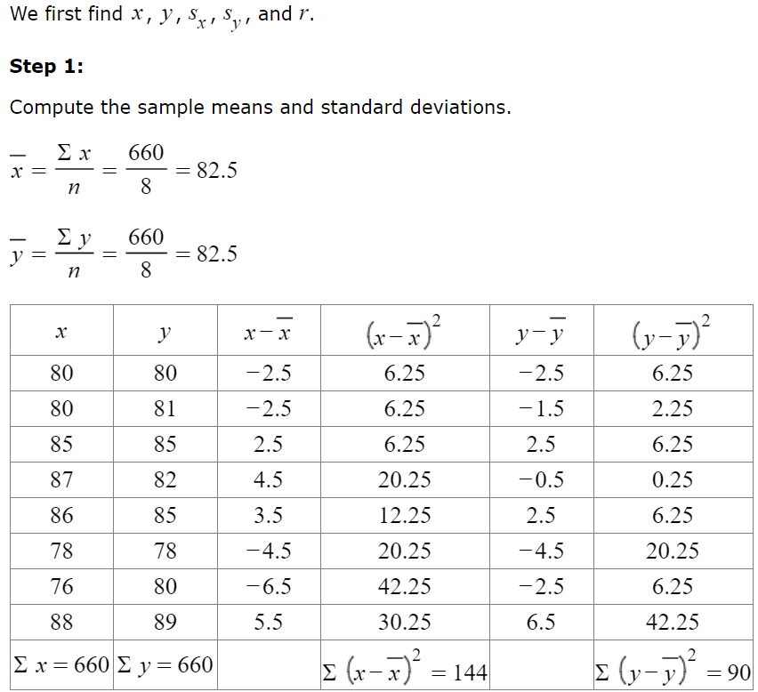
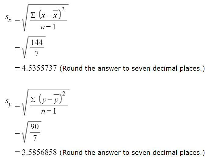
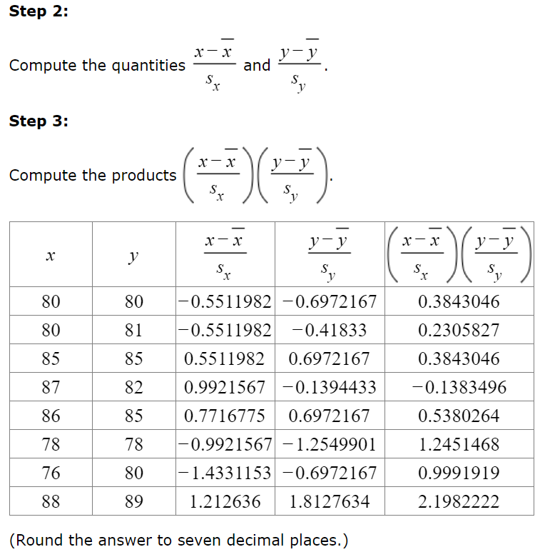
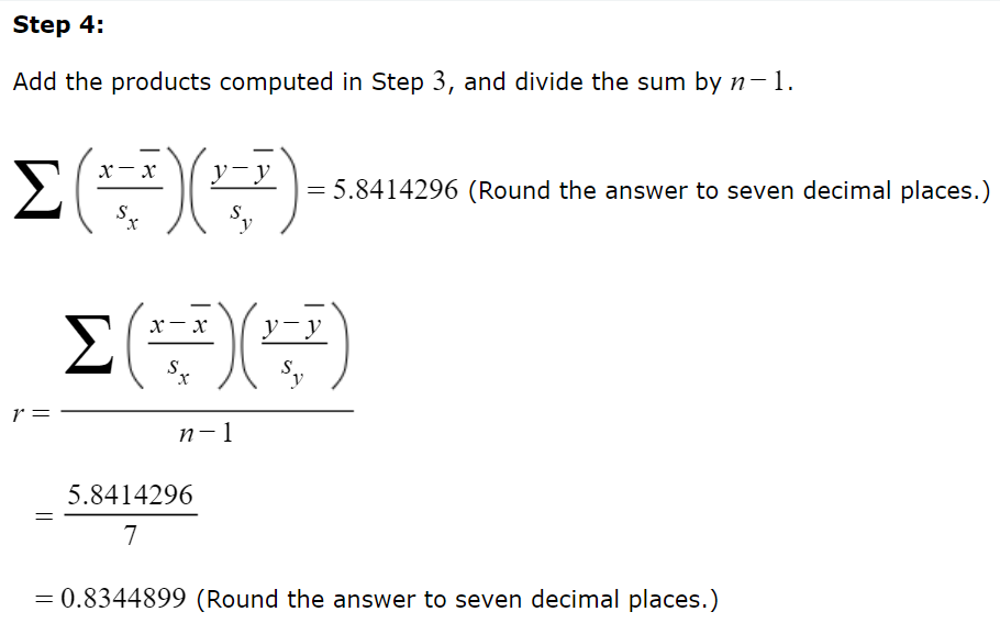
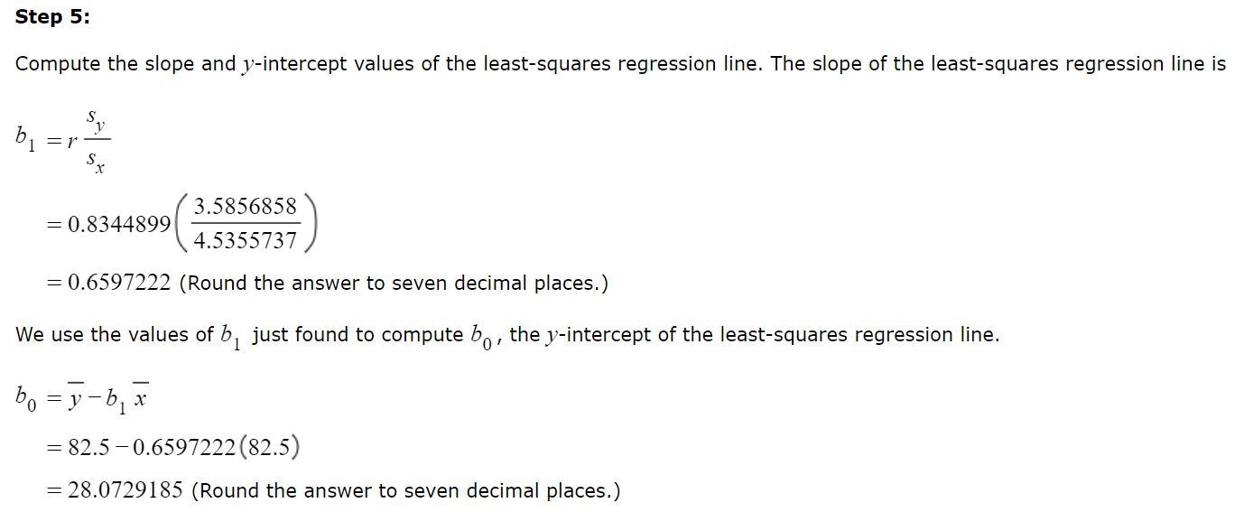
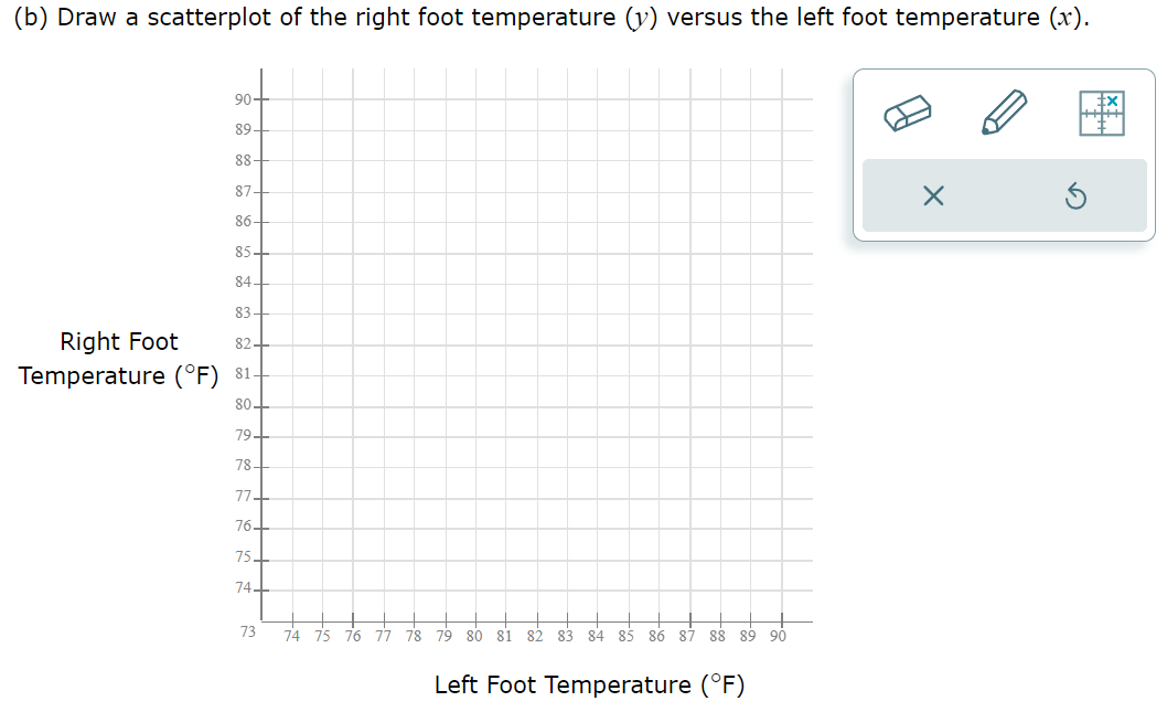
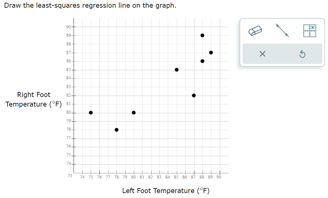
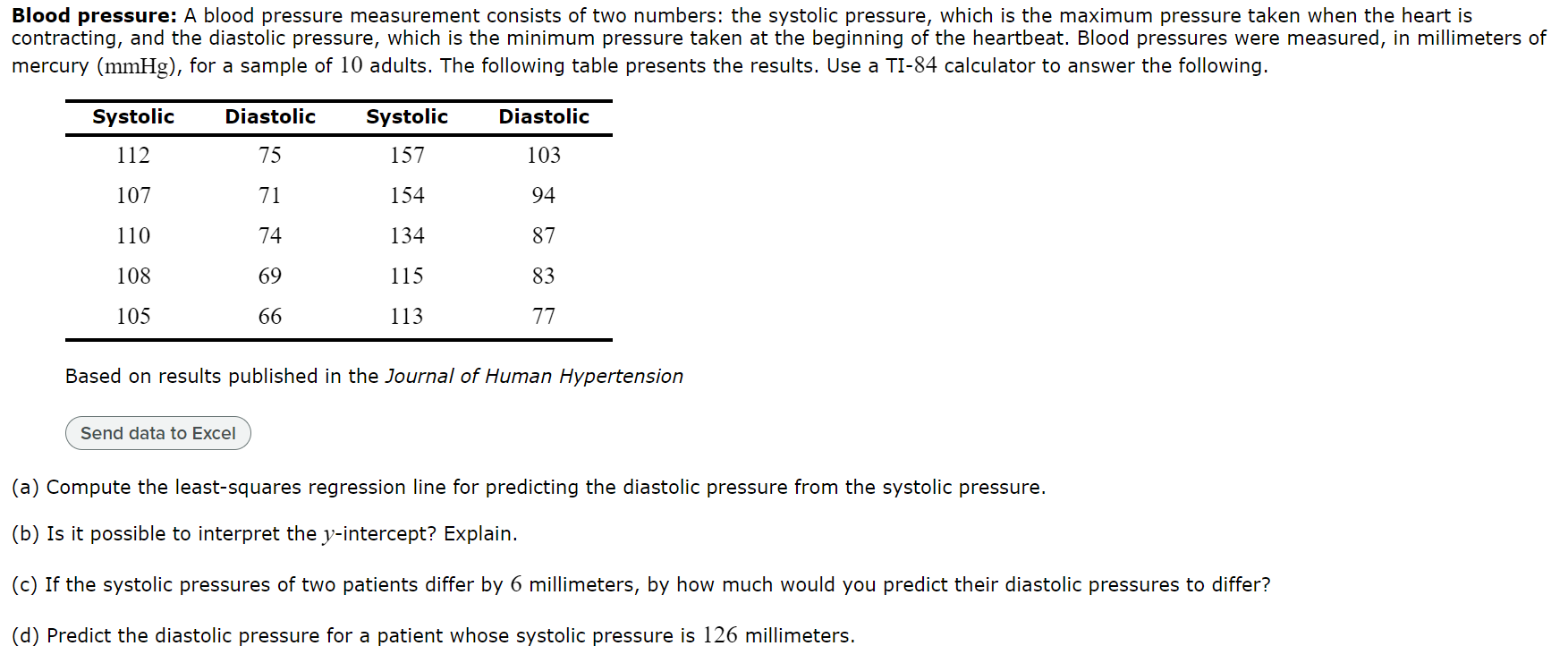
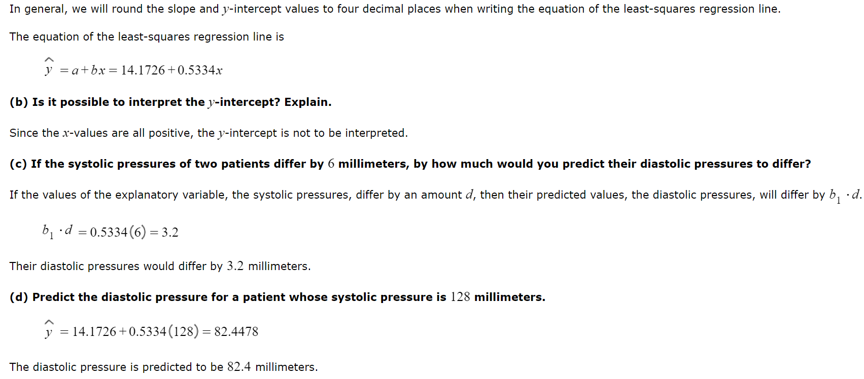
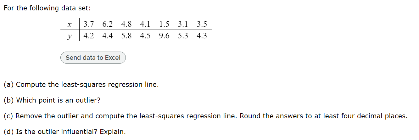
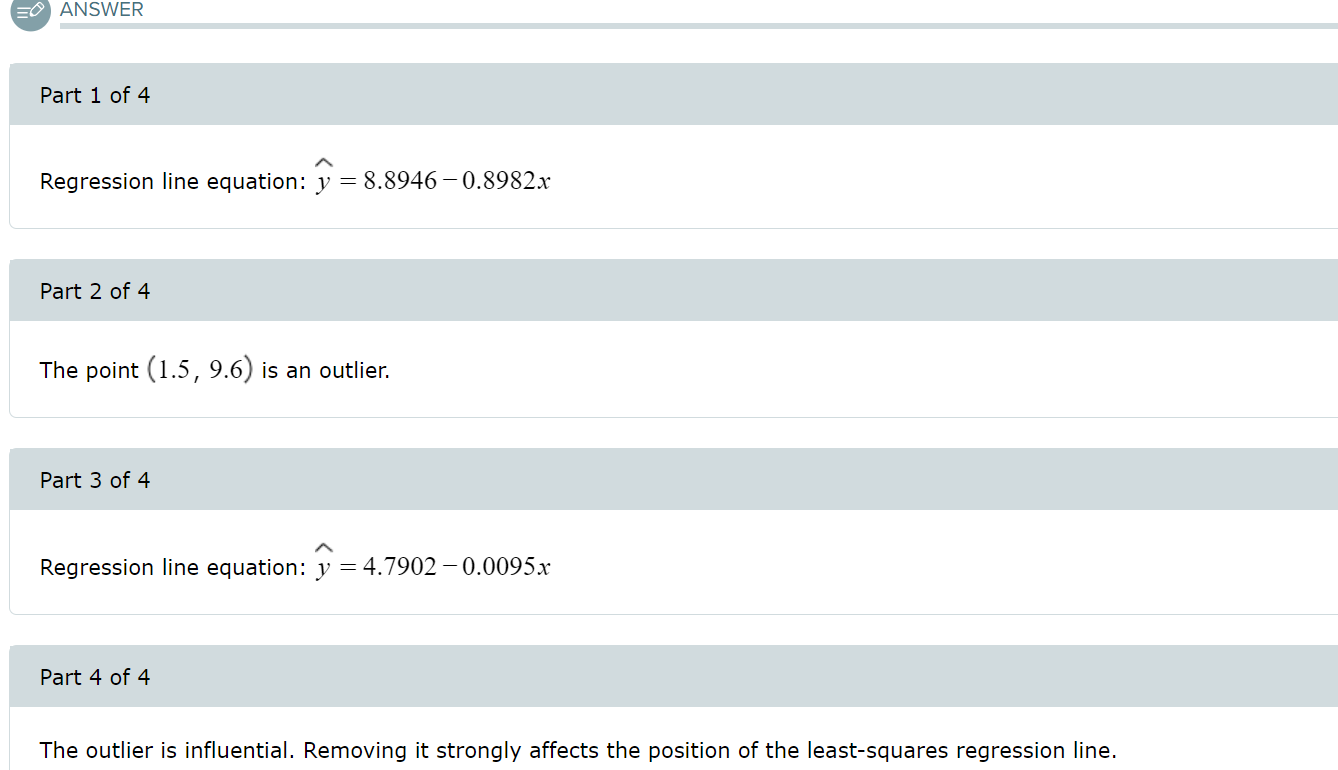
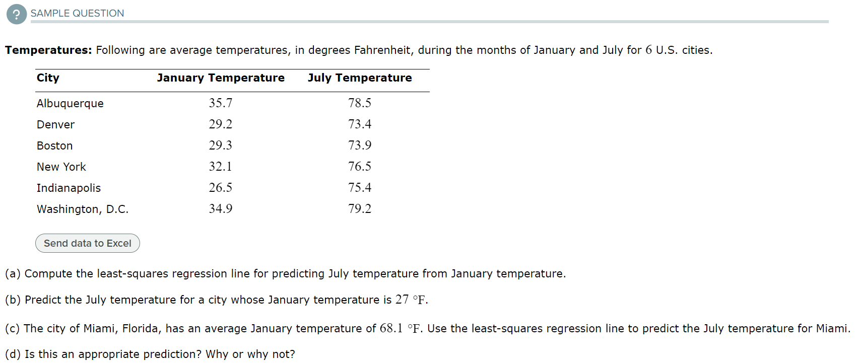
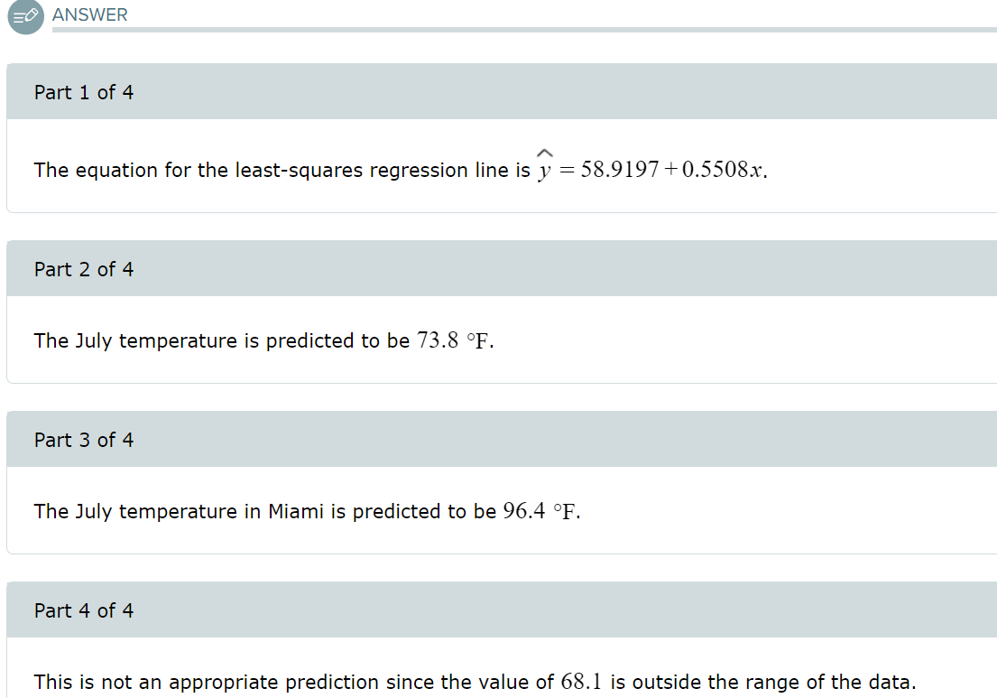
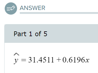
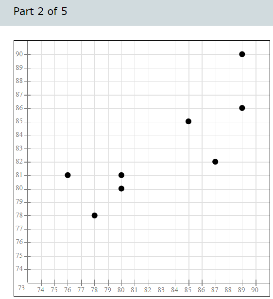
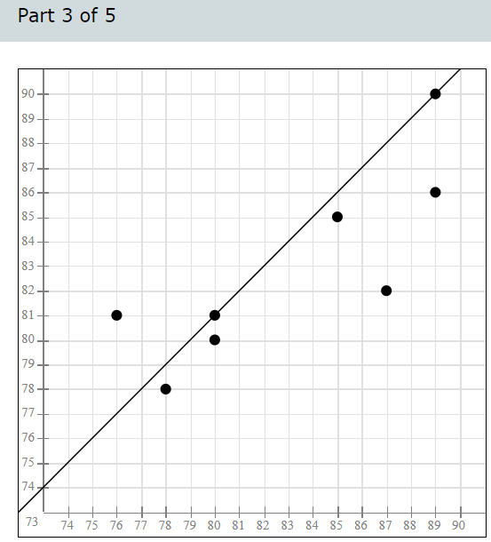
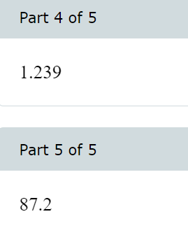
(a) Compute the least-squares regression line for predicting the right foot temperatures from the left foot temperature. Round the slope and y-intercept values to four decimal places. = Regression line equation: y Foot temperatures: Foot ulcers are a common problem for people with diabetes. Higher skin temperatures on the foot indicate an increased risk of ulcers. In a study performed at the Colorado School of Mines, skin temperatures on both feet were measured, in degrees Fahrenheit, for 8 diabetic patients. The results are presented in the following table. Left Foot Right Foot 80 80 80 81 85 85 87 82 86 85 78 78 76 88 888 80 89 (a) Compute the least-squares regression line for predicting the right foot temperatures from the left foot temperature. Equation of the Least-squares Regression Line Given ordered pairs (x, y), with sample means x and y, sample standard deviations and regression line for predicting y from x is Sx where b S S ' =r is the slope and boy-bx is the y-intercept. x and correlation coefficient r, the equation of the least-squares y' We first find x, y, Sx, S, and r. Step 1: Compute the sample means and standard deviations. 660 - x = 82.5 n 8 - n 660 = = 82.5 8 - y X-X (x-x) - y-y (y-5) 60 80 80 -2.5 6.25 -2.5 6.25 80 81 -2.5 6.25 -1.5 2.25 85 85 2.5 6.25 2.5 6.25 87 82 4.5 20.25 -0.5 0.25 86 85 3.5 12.25 2.5 6.25 78 78 -4.5 20.25 -4.5 20.25 76 80 -6.5 42.25 -2.5 6.25 88 89 5.5 30.25 6.5 42.25 x = 660 y = 660 (x-x) = 144 (y-1)=90 = - = 2 (x-5) 144 n-1 7 = 4.5355737 (Round the answer to seven decimal places.) = = (y y) 90 7 n-1 = 3.5856858 (Round the answer to seven decimal places.) Step 2: X-X Compute the quantities y-y and S S y Step 3: Compute the products x x y-y ()(+) S S y X-X y-y X-X y-y * x y S x Sy S x Sy 88 80 80 80 -0.5511982 -0.6972167 81 -0.5511982 -0.41833 0.3843046 0.2305827 85 85 0.5511982 0.6972167 0.3843046 87 82 0.9921567 -0.1394433 -0.1383496 86 85 0.7716775 0.6972167 0.5380264 78 78 -0.9921567 -1.2549901 1.2451468 76 80 -1.4331153 -0.6972167 0.9991919 88 89 1.212636 1.8127634 2.1982222 (Round the answer to seven decimal places.) Step 4: Add the products computed in Step 3, and divide the sum by n1. X-X y-y = 5.8414296 (Round the answer to seven decimal places.) S S y X-X S x r = y-y S y = n-1 5.8414296 7 0.8344899 (Round the answer to seven decimal places.) Step 5: Compute the slope and y-intercept values of the least-squares regression line. The slope of the least-squares regression line is =r 3.5856858 = 0.8344899 4.5355737 = 0.6597222 (Round the answer to seven decimal places.) We use the values of b just found to compute bo, the y-intercept of the least-squares regression line. b = y-b x = 82.5-0.6597222 (82.5) = 28.0729185 (Round the answer to seven decimal places.) Step 6: Compute the equation of the least-squares regression line. In general, we will round the slope and y-intercept values to four decimal places when writing the equation of the least-squares regression line. The equation of the least-squares regression line is y bo+bx 28.0729+0.6597x (b) Draw a scatterplot of the right foot temperature (y) versus the left foot temperature (x). 90- 89 88- 87- 86- 85 84- 83- 82. Right Foot Temperature (F) 81- 80- 79- 78- 77 76- 75. 74 73 74 75 76 77 78 79 80 81 82 83 84 85 86 87 88 89 90 Left Foot Temperature (F) Draw the least-squares regression line on the graph. 90- 89- 88- 87- 86 85. 84- 83- 82 Right Foot Temperature (F) 81. 80- 79- 78- 77- 76- 75- 74 73 74 75 76 77 78 79 80 81 82 83 84 85 86 87 88 89 90 Left Foot Temperature (F) (c) If the left foot temperatures of two patients differ by 3 degrees, by how much would you predict their right foot temperatures to differ? Round the answer to three decimal places. The right foot temperatures would differ by degrees. Foot temperatures: Foot ulcers are a common problem for people with diabetes. Higher skin temperatures on the foot indicate an increased risk of ulcers. In a study performed at the Colorado School of Mines, skin temperatures on both feet were measured, in degrees Fahrenheit, for 8 diabetic patients. The results are presented in the following table. Left Foot Right Foot 78 78 89 87 2 89 87 80 L 90 85 82 80 88 89 85 76 81 Blood pressure: A blood pressure measurement consists of two numbers: the systolic pressure, which is the maximum pressure taken when the heart is contracting, and the diastolic pressure, which is the minimum pressure taken at the beginning of the heartbeat. Blood pressures were measured, in millimeters of mercury (mmHg), for a sample of 10 adults. The following table presents the results. Use a TI-84 calculator to answer the following. Systolic Diastolic Systolic Diastolic 112 75 157 103 107 71 154 94 110 74 134 87 108 69 115 83 105 66 113 77 Based on results published in the Journal of Human Hypertension Send data to Excel (a) Compute the least-squares regression line for predicting the diastolic pressure from the systolic pressure. (b) Is it possible to interpret the y-intercept? Explain. (c) If the systolic pressures of two patients differ by 6 millimeters, by how much would you predict their diastolic pressures to differ? (d) Predict the diastolic pressure for a patient whose systolic pressure is 126 millimeters. Blood pressure: A blood pressure measurement consists of two numbers: the systolic pressure, which is the maximum pressure taken when the heart is contracting, and the diastolic pressure, which is the minimum pressure taken at the beginning of the heartbeat. Blood pressures were measured, in millimeters of mercury (mmHg), for a sample of 10 adults. The following table presents the results. Use a TI-84 calculator to answer the following. Systolic Diastolic Systolic Diastolic 133 91 105 66 112 75 157 103 107 71 154 94 110 74 134 87 108 69 115 83 83 Compute the least-squares regression line for predicting the diastolic pressure from the systolic pressure. Round the slope and y-intercept to at least four decimal places. Regression line equation: y In general, we will round the slope and y-intercept values to four decimal places when writing the equation of the least-squares regression line. The equation of the least-squares regression line is y=a+bx=14.1726+0.5334x (b) Is it possible to interpret the y-intercept? Explain. Since the x-values are all positive, the y-intercept is not to be interpreted. (c) If the systolic pressures of two patients differ by 6 millimeters, by how much would you predict their diastolic pressures to differ? If the values of the explanatory variable, the systolic pressures, differ by an amount d, then their predicted values, the diastolic pressures, will differ by b d. b.d= 0.5334 (6)=3.2 Their diastolic pressures would differ by 3.2 millimeters. (d) Predict the diastolic pressure for a patient whose systolic pressure is 128 millimeters. y=14.1726+0.5334 (128) = 82.4478 The diastolic pressure is predicted to be 82.4 millimeters. For the following data set: x 3.6 5.7 4.1 3.3 1.5 3.4 3.1 Part: 0 / 4 Part 1 of 4 y 4.2 4.7 5.4 4.8 9.3 5.5 4.5 Send data to Excel (a) Compute the least-squares regression line. Round the answers to at least four decimal places. Regression line equation: y = For the following data set: x 3.7 6.2 4.8 4.1 1.5 3.1 3.5 y 4.2 4.4 5.8 4.5 9.6 9.6 5.3 4.3 Send data to Excel (a) Compute the least-squares regression line. (b) Which point is an outlier? (c) Remove the outlier and compute the least-squares regression line. Round the answers to at least four decimal places. (d) Is the outlier influential? Explain. ANSWER Part 1 of 4 Regression line equation: y = 8.8946-0.8982x Part 2 of 4 The point (1.5, 9.6) is an outlier. Part 3 of 4 Regression line equation: y = 4.7902 -0.0095x Part 4 of 4 The outlier is influential. Removing it strongly affects the position of the least-squares regression line. Temperatures: Following are average temperatures, in degrees Fahrenheit, during the months of January and July for 6 U.S. cities. City Detroit Albuquerque Atlanta Chicago Denver Boston Send data to Excel January Temperature July Temperature 24.5 73.5 35.7 78.5 42.7 80.0 22.0 73.3 29.2 73.4 29.3 73.9 (a) Compute the least-squares regression line for predicting July temperature from January temperature. The equation for the least-squares regression line is y = . Round the slope and y-intercept to four decimal places as needed. ? SAMPLE QUESTION Temperatures: Following are average temperatures, in degrees Fahrenheit, during the months of January and July for 6 U.S. cities. City Albuquerque Denver January Temperature July Temperature 35.7 78.5 29.2 73.4 29.3 73.9 32.1 76.5 Indianapolis 26.5 Washington, D.C. 34.9 75.4 79.2 Boston New York Send data to Excel (a) Compute the least-squares regression line for predicting July temperature from January temperature. (b) Predict the July temperature for a city whose January temperature is 27 F. (c) The city of Miami, Florida, has an average January temperature of 68.1 F. Use the least-squares regression line to predict the July temperature for Miami. (d) Is this an appropriate prediction? Why or why not? ANSWER Part 1 of 4 The equation for the least-squares regression line is y = 58.9197 +0.5508x. Part 2 of 4 The July temperature is predicted to be 73.8 F. Part 3 of 4 The July temperature in Miami is predicted to be 96.4 F. Part 4 of 4 This is not an appropriate prediction since the value of 68.1 is outside the range of the data. E ANSWER Part 1 of 5 y = 31.4511 +0.6196x Part 2 of 5 90+ 89 88 87- 86- 85 84 83 82 81 80 79 78. 77 76 75+ 74+ 73 74 75 76 77 78 79 80 81 82 83 84 85 86 87 88 89 90 Part 3 of 5 190+ 89- 88 87 86- 85 84 83 82 81 80- 79 78 77 76 75 74 73 74 75 76 77 78 79 80 81 82 83 84 85 86 87 88 89 90 Part 4 of 5 1.239 Part 5 of 5 87.2