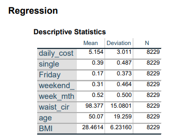
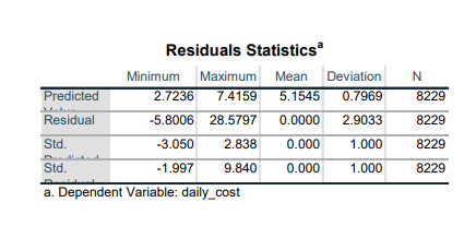
A good friend of yours works as a financial analyst in a hospital that has an emergency care unit. Triage nurses are well trained at allocating care based on the severity of injuries, and the hospital is proud of its low mortality rate. Your friend is acutely aware of pressure on the hospital to try and manage treatment costs and so she is trying to understand whether there are any predictors (besides apparent injuries) which may help staff to manage the cost of treating patients who arrive at the casualty unit. She assesses 8229 cases over the past three years and creates the regression model detailed in the SPSS output below.

Knowing that you have recently improved your skills as an analyst, she asks you to critique her approach and model.

The model consists of the following variables:

? Daily cost- the cost of treating a patient in USD thousand

? Single- whether the patient is single or married

? Friday- a dummy variable indicating day of treatment

? Weekend SS -a dummy variable indicating day of treatment

? Waist - a measure of the patients girth on arrival

? Age- in years

? BMI- estimated Body Mass Index of patient on arrival

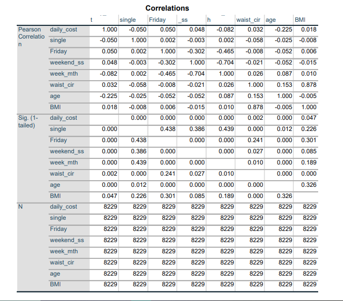
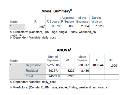
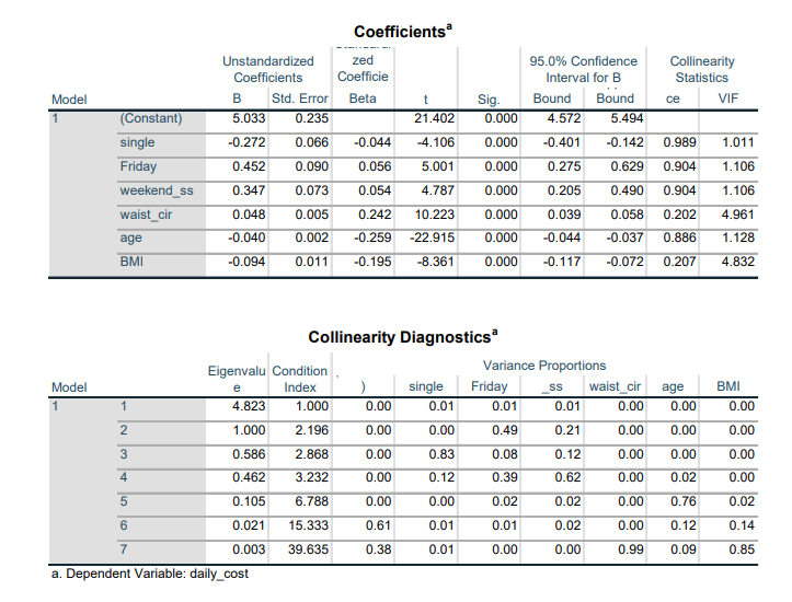
Using the SPSS outputs , discuss the efficacy of the model and any potential regression problems in the model. Make recommendations as to what you would change in her approach.

\fCorrelations single Friday SS h waist cir age BMI Pearson daily_cost 1.000 -0.050 0.050 0.048 -0.082 0.032 -0.225 0.018 Correlatio single -0.050 1.000 0.002 -0.003 0.002 -0.058 -0.025 -0.008 n Friday 0.050 0.002 1.000 -0.302 -0.465 -0.008 -0.052 0.006 weekend ss 0.048 -0.003 -0.302 1.000 -0.704 -0.021 -0.052 -0.015 week mth -0.082 0.002 -0.465 -0.704 1.000 0.026 0.087 0.010 waist cir 0.032 -0.058 -0.008 -0.021 0.026 1.000 0.153 0.878 age -0.225 -0.025 -0.052 -0.052 0.087 0.153 1.000 -0.005 BM 0.018 -0.008 0.006 -0.015 0.010 0.878 -0.005 1.000 Sig. (1- daily_cost 0.000 0.000 0.000 0.000 0.002 0.000 0.047 tailed) single 0.000 0.438 0.386 0.439 0.000 0.012 0.226 Friday 0.000 0.438 0.000 0.000 0.241 0.000 0.301 weekend ss 0.000 0.386 0.000 0.000 0.027 0.000 0.085 week mth 0.000 0.439 0.000 0.000 0.010 0.000 0.189 waist cir 0.002 0.000 0.241 0.027 0.010 0.000 0.000 age 0.000 0.012 0.000 0.000 0.000 0.000 0.326 BMI 0.047 0.226 0.301 0.085 0.189 0.000 0.326 N daily_cost 8229 8229 8229 8229 8229 8229 8229 8229 single 8229 8229 8229 8229 8229 8229 8229 8229 Friday 8229 8229 8229 8229 8229 8229 8229 8229 weekend ss 8229 8229 8229 8229 8229 8229 8229 8229 week mth 8229 8229 8229 8229 8229 8229 8229 8229 waist_cir 8229 8229 8229 8229 8229 8229 8229 8229 age 8229 8229 8229 8229 8229 8229 8229 8229 BMI 8229 8229 8229 8229 8229 8229 8229 8229Model Summary Adjusted of the Durbin- Model R R Square R Square Estimate Watson 1 .265 0.070 0.069 2.904 1.923 a. Predictors: (Constant), BMI, age, single, Friday, weekend ss, sriet alF b. Dependent Variable: daily_cost ANOVA Sum of Mean Model Squares di Square F Sig. Regression 5225.505 6 870.917 103.244 000 Residual 69357.1 8222 8.436 Total 74582.6 8228 a. Dependent Variable: daily_cost b. Predictors: (Constant), BMI, age, single, Friday, weekend_ss, waist cirCoefficients Unstandardized zed 95.0% Confidence Collinearity Coefficients Coefficie Interval for B Statistics Model B Std. Error Beta Sig. Bound Bound ce VIF (Constant) 5.033 0.235 21.402 0.000 4.572 5.494 single -0.272 0.066 -0.044 4.106 0.000 -0.401 -0.142 0.989 1.011 Friday 0.452 0.090 0.056 5.001 0.000 0.275 0.629 0.904 1.106 weekend ss 0.347 0.073 0.054 4.787 0.000 0.205 0.490 0.904 1.106 waist cir 0.048 0.005 0.242 10.223 0.000 0.039 0.058 0.202 4.961 age -0.040 0.002 -0.259 -22.915 0.000 -0.044 -0.037 0.886 1.128 BMI -0.094 0.011 -0.195 -8.361 0.000 -0.117 -0.072 0.207 4.832 Collinearity Diagnostics Eigenvaluendition Variance Proportions Model e Index single Friday SS waist cir age BM 4.823 1.000 0.00 0.01 0.01 0.01 0.00 0.00 0.00 1.000 2.196 0.00 0.00 0.49 0.21 0.00 0.00 0.00 0.586 2.868 0.00 0.83 0.08 0.12 0.00 0.00 0.00 0.462 3.232 0.00 0.12 0.39 0.62 0.00 0.02 0.00 5 0.105 6.788 0.00 0.00 0.02 0.02 0.00 0.76 0.02 6 0.021 15.333 0.61 0.01 0.01 0.02 0.00 0.12 0.14 7 0.003 39.635 0.38 0.01 0.00 0.00 0.99 0.09 0.85 a. Dependent Variable: daily_cost\f