a. How successful is the yield curve at predicting recessions?
b. What matters most the level of the term spread, the change in the spread, or the level of short term interest rates?
c. why a yield curve inversion should lead to a recession.
2. Dick Berner (Morgan Stanley) is a bit more skeptical about the predictive power of the yield curve. Does he just not understand Estrellas overwhelming evidence, or does his skepticism rest on solid reasoning?
3. How is the U.S. yield curve currently sloped? What does it affect your forecast of economic activity?


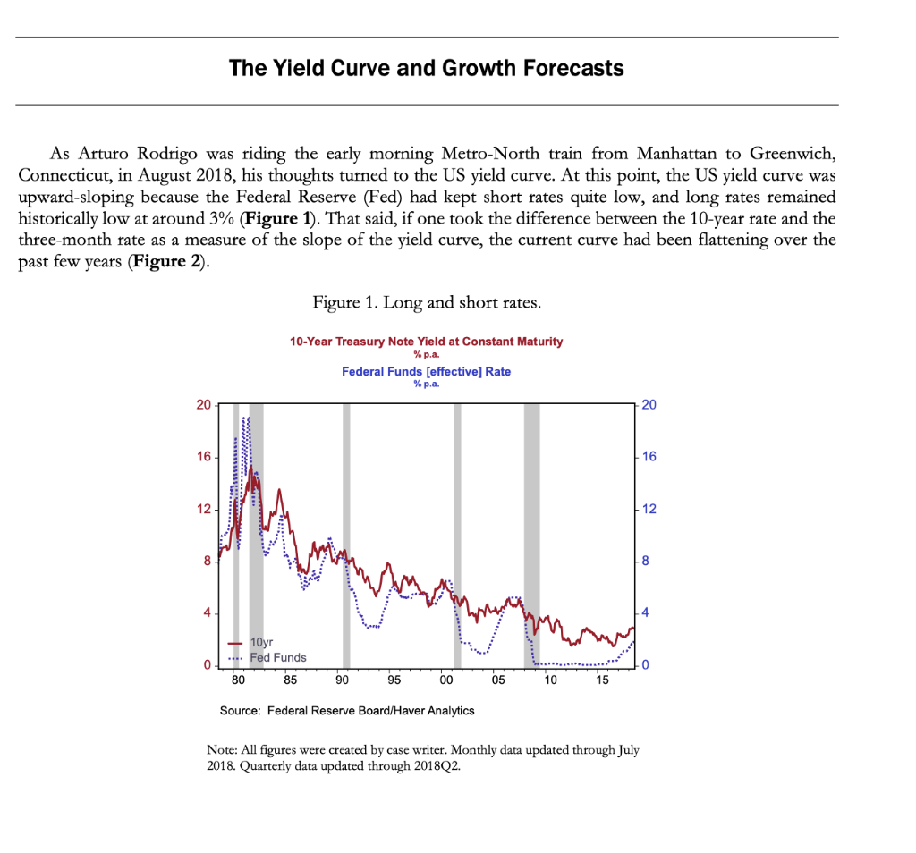
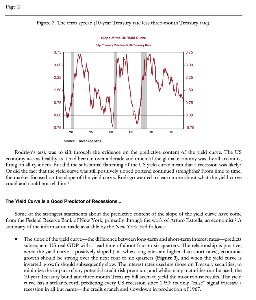
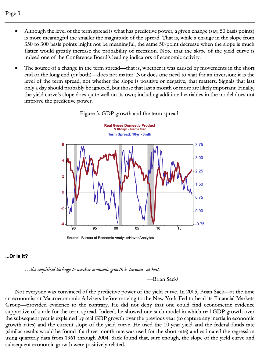
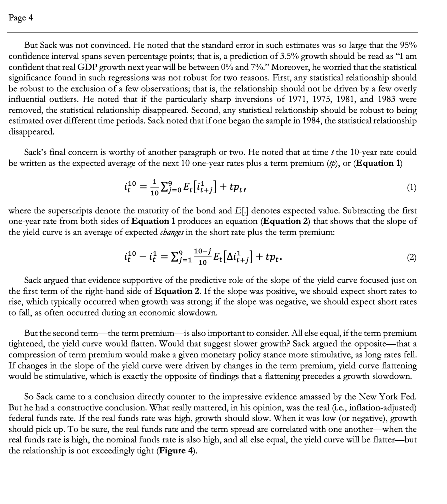
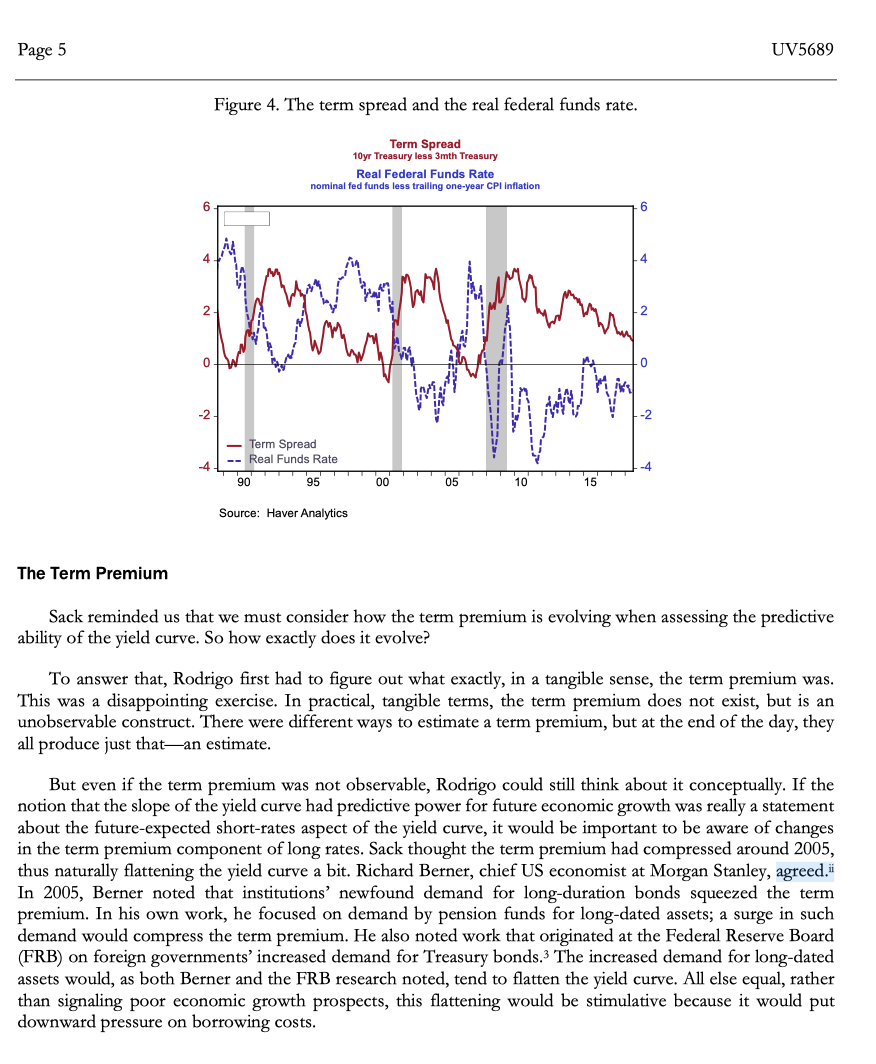
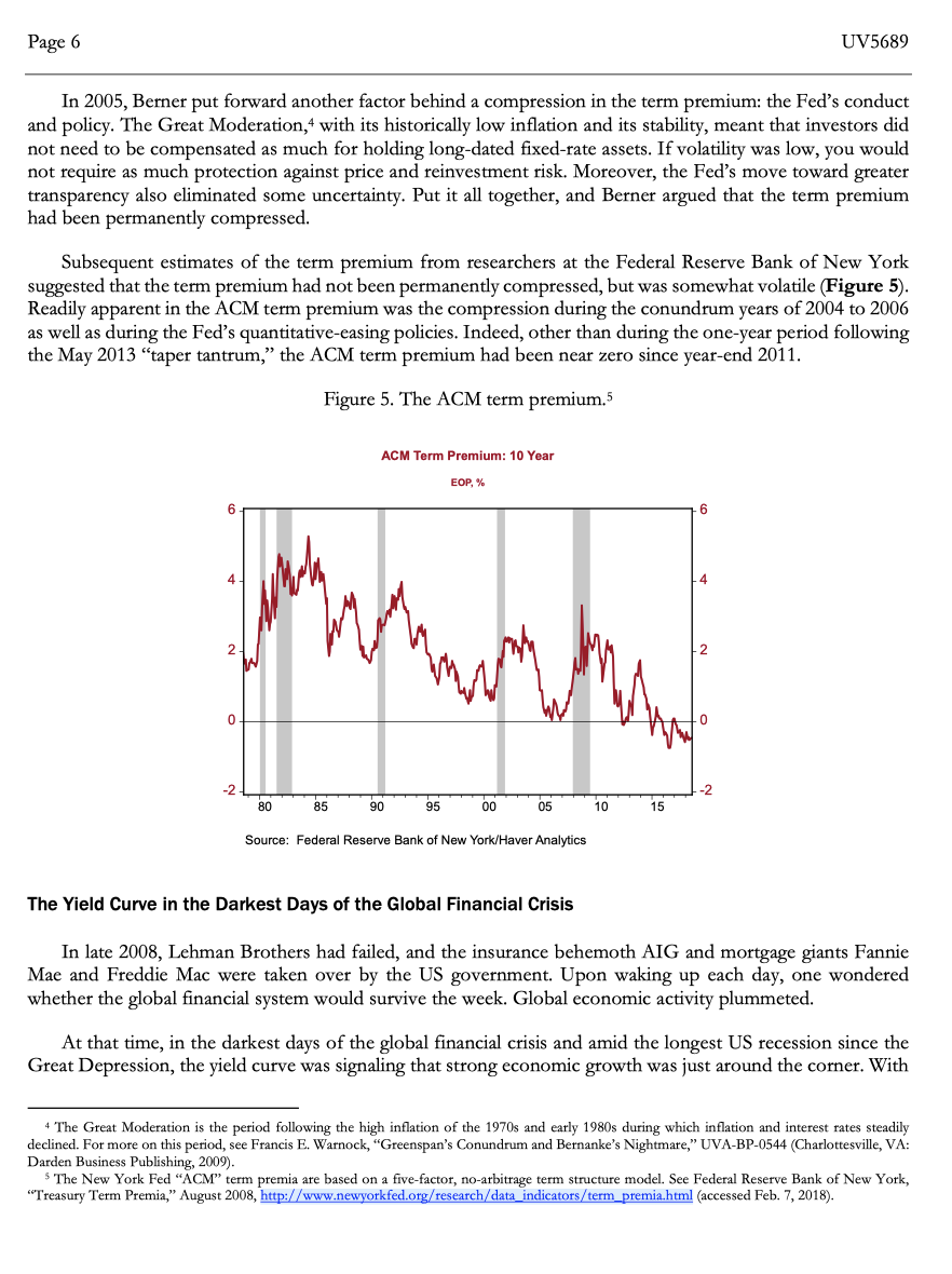
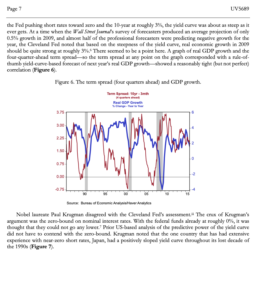
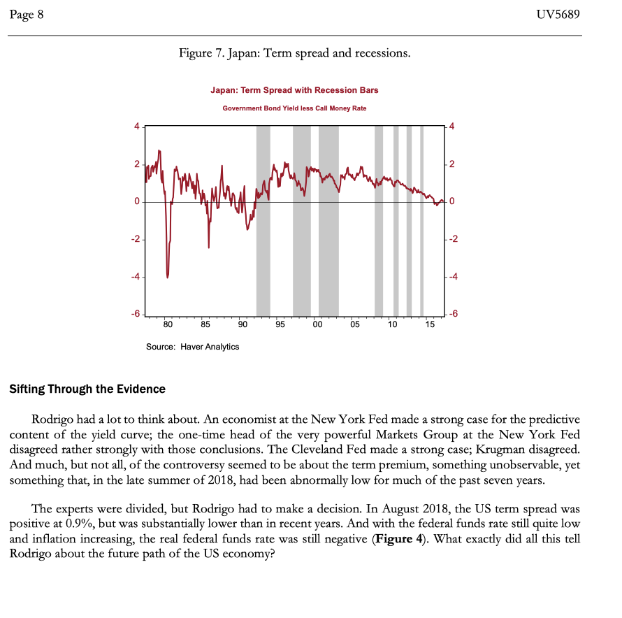
The Yield Curve and Growth Forecasts As Arturo Rodrigo was riding the early morning Metro-North train from Manhattan to Greenwich, Connecticut, in August 2018, his thoughts turned to the US yield curve. At this point, the US yield curve was upward-sloping because the Federal Reserve (Fed) had kept short rates quite low, and long rates remained historically low at around 3% (Figure 1). That said, if one took the difference between the 10-year rate and the three-month rate as a measure of the slope of the yield curve, the current curve had been flattening over the past few years (Figure 2). Figure 1. Long and short rates. 10-Year Treasury Note Yield at Constant Maturity %p.a. Federal Funds [effective] Rate % p.a. 20 20 16 16 12 12 8 8 4 0 10yr Fed Funds 80 85 0 90 95 00 05 10 15 Source: Federal Reserve Board/Haver Analytics Note: All figures were created by case writer. Monthly data updated through July 2018. Quarterly data updated through 2018Q2. Page 2 Figure 2. The term spread (10-year Treasury rate less three-month Treasury rate). Slope of the US Yield Curve 10yr Treasury Rate less 3mth Treasury Rate 3.75 3.75 3.00 3.00 2.25 -2.25 1.50 1.50 0.75 0.75 0.00 0.00 -0.75 -0.75 90 95 05 15 Source: Haver Analytics Rodrigo's task was to sift through the evidence on the predictive content of the yield curve. The US economy was as healthy as it had been in over a decade and much of the global economy was, by all accounts, firing on all cylinders. But did the substantial flattening of the US yield curve mean that a recession was likely? Or did the fact that the yield curve was still positively sloped portend continued strenghths? From time to time, the market focused on the slope of the yield curve. Rodrigo wanted to learn more about what the yield curve could and could not tell him.1 The Yield Curve is a Good Predictor of Recessions... Some of the strongest statements about the predictive content of the slope of the yield curve have come from the Federal Reserve Bank of New York, primarily through the work of Arturo Estrella, an economist.2 A summary of the information made available by the New York Fed follows: The slope of the yield curvethe difference between long-term and short-term interest ratespredicts subsequent US real GDP with a lead time of about four to six quarters. The relationship is positive; when the yield curve is positively sloped (1.e., when long rates are higher than short rates), economic growth should be strong over the next four to six quarters (Figure 3), and when the yield curve is inverted, growth should subsequently slow. The interest rates used are those on Treasury securities, to minimize the impact of any potential credit risk premium, and while many maturities can be used, the 10-year Treasury bond and three-month Treasury bill seem to yield the most robust results. The yield curve has a stellar record, predicting every US recession since 1950; its only "false" signal foresaw a recession in all but namethe credit crunch and slowdown in production of 1967. Page 3 . Although the level of the term spread is what has predictive power, a given change (say, 50 basis points) is more meaningful the smaller the magnitude of the spread. That is, while a change in the slope from 350 to 300 basis points might not be meaningful, the same 50-point decrease when the slope is much flatter would greatly increase the probability of recession. Note that the slope of the yield curve is indeed one of the Conference Board's leading indicators of economic activity. The source of a change in the term spreadthat is, whether it was caused by movements in the short end or the long end (or both)does not matter. Nor does one need to wait for an inversion; it is the level of the term spread, not whether the slope is positive or negative, that matters. Signals that last only a day should probably be ignored, but those that last a month or more are likely important. Finally, the yield curve's slope does quite well on its own; including additional variables in the model does not improve the predictive power. . Figure 3. GDP growth and the term spread. Real Gross Domestic Product % Change - Year to Year Term Spread: 10yr - 3mth 3.75 -3.00 2.25 2 1.50 0 0.75 -2 0.00 -0.75 90 95 00 05 10 15 Source: Bureau of Economic Analysis/Haver Analytics ...Or Is It? ... the empirical linkage to weaker economic growth is tenuous, at best. Brian Sacki Not everyone was convinced of the predictive power of the yield curve. In 2005, Brian Sackat the time an economist at Macroeconomic Advisers before moving to the New York Fed to head its Financial Markets Group-provided evidence to the contrary. He did not deny that one could find econometric evidence supportive of a role for the term spread. Indeed, he showed one such model in which real GDP growth over the subsequent year is explained by real GDP growth over the previous year (to capture any inertia in economic growth rates) and the current slope of the yield curve. He used the 10-year yield and the federal funds rate (similar results would be found if a three-month rate was used for the short rate) and estimated the regression using quarterly data from 1961 through 2004. Sack found that, sure enough, the slope of the yield curve and subsequent economic growth were positively related. Page 4 But Sack was not convinced. He noted that the standard error in such estimates was so large that the 95% confidence interval spans seven percentage points; that is, a prediction of 3.5% growth should be read as I am confident that real GDP growth next year will be between 0% and 7%. Moreover, he worried that the statistical significance found in such regressions was not robust for two reasons. First, any statistical relationship should be robust to the exclusion of a few observations; that is, the relationship should not be driven by a few overly influential outliers. He noted that if the particularly sharp inversions of 1971, 1975, 1981, and 1983 were removed, the statistical relationship disappeared. Second, any statistical relationship should be robust to being estimated over different time periods. Sack noted that if one began the sample in 1984, the statistical relationship disappeared. Sack's final concern is worthy of another paragraph or two. He noted that at time t the 10-year rate could be written as the expected average of the next 10 one-year rates plus a term premium (Ip), or (Equation 1) it = --%%-o E[[it+j] + tpt1 (1) where the superscripts denote the maturity of the bond and E[:] denotes expected value. Subtracting the first one-year rate from both sides of Equation 1 produces an equation (Equation 2) that shows that the slope of the yield curve is an average of expected changes in the short rate plus the term premium: i i = 29-1100 E [Ai{+j] + tpz. (2) Sack argued that evidence supportive of the predictive role of the slope of the yield curve focused just on the first term of the right-hand side of Equation 2. If the slope was positive, we should expect short rates to rise, which typically occurred when growth was strong; if the slope was negative, we should expect short rates to fall, as often occurred during an economic slowdown. But the second termthe term premiumis also important to consider. All else equal, if the term premium tightened, the yield curve would flatten. Would that suggest slower growth? Sack argued the oppositethat a compression of term premium would make a given monetary policy stance more stimulative, as long rates fell. If changes in the slope of the yield curve were driven by changes in the term premium, yield curve flattening would be stimulative, which is exactly the opposite of findings that a flattening precedes a growth slowdown. So Sack came to a conclusion directly counter to the impressive evidence amassed by the New York Fed. But he had a constructive conclusion. What really mattered, in his opinion, was the real (i.e., inflation-adjusted) federal funds rate. If the real funds rate was high, growth should slow. When it was low or negative), growth should pick up. To be sure, the real funds rate and the term spread are correlated with one anotherwhen the real funds rate is high, the nominal funds rate is also high, and all else equal, the yield curve will be flatterbut the relationship is not exceedingly tight (Figure 4). Page 5 UV5689 Figure 4. The term spread and the real federal funds rate. Term Spread 10yr Treasury less 3mth Treasury Real Federal Funds Rate nominal fed funds less trailing one-year CPI Inflation 6 4 2 -2 - Term Spread Real Funds Rate -4 90 95 00 05 10 15 Source: Haver Analytics The Term Premium Sack reminded us that we must consider how the term premium is evolving when assessing the predictive ability of the yield curve. So how exactly does it evolve? To answer that, Rodrigo first had to figure out what exactly, in a tangible sense, the term premium was. This was a disappointing exercise. In practical, tangible terms, the term premium does not exist, but is an unobservable construct. There were different ways to estimate a term premium, but at the end of the day, they all produce just thatan estimate. But even if the term premium was not observable, Rodrigo could still think about it conceptually. If the notion that the slope of the yield curve had predictive power for future economic growth was really a statement about the future-expected short-rates aspect of the yield curve, it would be important to be aware of changes in the term premium component of long rates. Sack thought the term premium had compressed around 2005, thus naturally flattening the yield curve a bit. Richard Berner, chief US economist at Morgan Stanley, agreed. In 2005, Berner noted that institutions' newfound demand for long-duration bonds squeezed the term premium. In his own work, he focused on demand by pension funds for long-dated assets; a surge in such demand would compress the term premium. He also noted work that originated at the Federal Reserve Board (FRB) on foreign governments' increased demand for Treasury bonds. The increased demand for long-dated assets would, as both Berner and the FRB research noted, tend to flatten the yield curve. All else equal, rather than signaling poor economic growth prospects, this flattening would be stimulative because it would put downward pressure on borrowing costs. Page 6 UV5689 In 2005, Berner put forward another factor behind a compression in the term premium: the Fed's conduct and policy. The Great Moderation, with its historically low inflation and its stability, meant that investors did not need to be compensated as much for holding long-dated fixed-rate assets. If volatility was low, you would not require as much protection against price and reinvestment risk. Moreover, the Fed's move toward greater transparency also eliminated some uncertainty. Put it all together, and Berner argued that the term premium had been permanently compressed. Subsequent estimates of the term premium from researchers at the Federal Reserve Bank of New York suggested that the term premium had not been permanently compressed, but was somewhat volatile (Figure 5). Readily apparent in the ACM term premium was the compression during the conundrum years of 2004 to 2006 as well as during the Fed's quantitative-easing policies. Indeed, other than during the one-year period following the May 2013 "taper tantrum, the ACM term premium had been near zero since year-end 2011. Figure 5. The ACM term premium.5 ACM Term Premium: 10 Year EOP, % 6 6 4 mark 2 -2 0 0 -2 -2 80 85 90 95 00 05 10 15 Source: Federal Reserve Bank of New York/Haver Analytics The Yield Curve in the Darkest Days of the Global Financial Crisis In late 2008, Lehman Brothers had failed, and the insurance behemoth AIG and mortgage giants Fannie Mae and Freddie Mac were taken over by the US government. Upon waking up each day, one wondered whether the global financial system would survive the week. Global economic activity plummeted. At that time, in the darkest days of the global financial crisis and amid the longest US recession since the Great Depression, the yield curve was signaling that strong economic growth was just around the corner. With 4 The Great Moderation is the period following the high inflation of the 1970s and early 1980s during which inflation and interest rates steadily declined. For more on this period, see Francis E. Warnock, "Greenspan's Conundrum and Bernanke's Nightmare," UVA-BP-0544 (Charlottesville, VA: Darden Business Publishing, 2009). The New York Fed "ACM" term premia are based on a five-factor, no-arbitrage term structure model. See Federal Reserve Bank of New York, "Treasury Term Premia," August 2008, http://www.newyorkfed.org/research/data_indicators/term_premia.html (accessed Feb. 7, 2018). Page 7 UV5689 the Fed pushing short rates toward zero and the 10-year at roughly 3%, the yield curve was about as steep as it ever gets. At a time when the Wall Street Journal's survey of forecasters produced an average projection of only 0.5% growth in 2009, and almost half of the professional forecasters were predicting negative growth for the year, the Cleveland Fed noted that based on the steepness of the yield curve, real economic growth in 2009 should be quite strong at roughly 3%. There seemed to be a point here. A graph of real GDP growth and the four-quarter-ahead term spreadso the term spread at any point on the graph corresponded with a rule-of- thumb yield-curve-based forecast of next year's real GDP growthshowed a reasonably tight (but not perfect) correlation (Figure 6). Figure 6. The term spread (four quarters ahead) and GDP growth. Term Spread: 10yr - 3mth (4 quarters ahead) Real GDP Growth % Change - Year to Year 3.75 6 3.00 2.25 2 1.50 0 0.75 -2 0.00 -0.75 -4 90 95 00 05 10 15 Source: Bureau of Economic Analysis/Haver Analytics Nobel laureate Paul Krugman disagreed with the Cleveland Fed's assessment.ii The crux of Krugman's argument was the zero-bound on nominal interest rates. With the federal funds already at roughly 0%, it was thought that they could not go any lower. Prior US-based analysis of the predictive power of the yield curve did not have to contend with the zero-bound. Krugman noted that the one country that has had extensive experience with near-zero short rates, Japan, had a positively sloped yield curve throughout its lost decade of the 1990s (Figure 7). Page 8 UV5689 Figure 7. Japan: Term spread and recessions. Japan: Term Spread with Recession Bars Government Bond Yield less Call Money Rate smo 0 10 -2 .-2 -4 -4 -6 80 85 90 95 00 05 10 15 Source: Haver Analytics Sifting Through the Evidence Rodrigo had a lot to think about. An economist at the New York Fed made a strong case for the predictive content of the yield curve; the one-time head of the very powerful Markets Group at the New York Fed disagreed rather strongly with those conclusions. The Cleveland Fed made a strong case; Krugman disagreed. And much, but not all, of the controversy seemed to be about the term premium, something unobservable, yet something that, in the late summer of 2018, had been abnormally low for much of the past seven years. The experts were divided, but Rodrigo had to make a decision. In August 2018, the US term spread was positive at 0.9%, but was substantially lower than in recent years. And with the federal funds rate still quite low and inflation increasing, the real federal funds rate was still negative (Figure 4). What exactly did all this tell Rodrigo about the future path of the US economy
