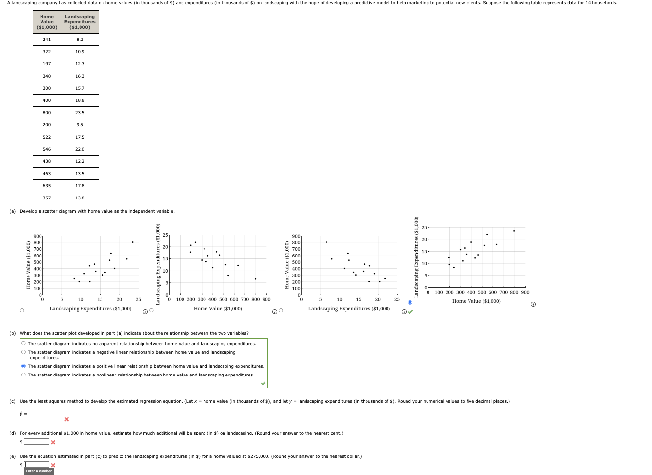
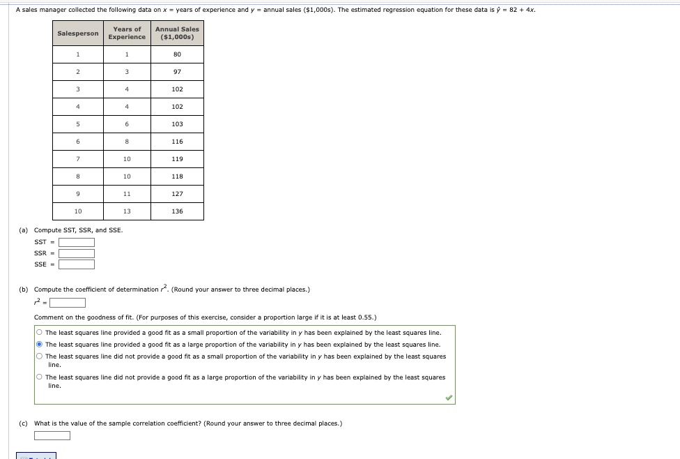
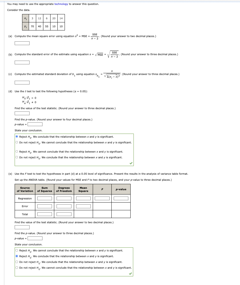
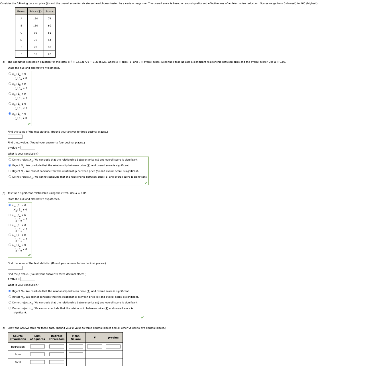
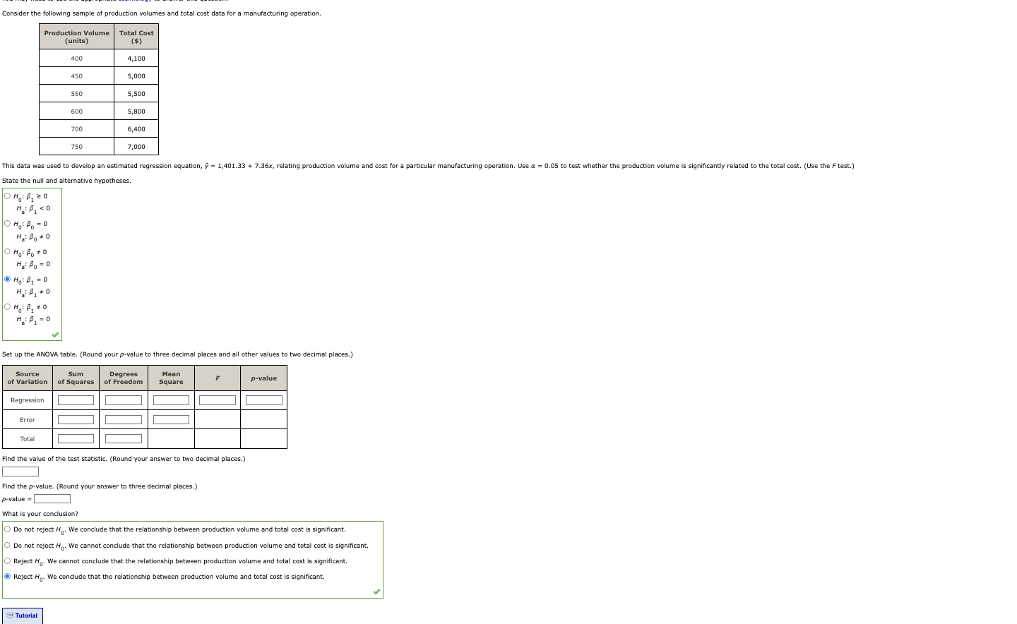
A landscaping company has collected data on home value r 14 households. Home Landscaping Value Expenditures ($1,000) ($1,000) 241 8 .2 322 10.9 197 12.3 340 16.3 300 15.7 400 18.8 800 23.5 200 522 17.5 546 22.0 438 12.2 463 13.5 635 17.8 357 13.8 (a) Develop a scatter diagram with home value as the independent variable. 900 900 800 700 20 8 700 600 15 600 Landscaping Expenditures ($1,000) 9 500 9 500 400 Landscaping Expenditures ($1,000 a 300 10 400 300 200 200 100 100 OL OL 0 100 200 300 400 500 600 700 800 900 10 15 20 25 0 100 200 300 400 500 600 700 800 900 10 15 20 Home Value ($1,000) Landscaping Expenditures ($1,000) Home Value ($1,000) Landscaping Expenditures ($1,000) (b) What does the scatter plot developed in part (a) indicate about the relationship between the two variables? O The scatter diagram indicates no apparer Blue and landscaping expenditures. The scatter diagram indicates a negative linear relationship between home value and landscaping expenditures. The scatter diagram indicates a positive linear relationship between home value and landscaping expenditures. The scatter diagram indicates a nonlinear relationship between home value and landscaping expenditures. (c) Use the least squares method to develop the estimated regression equation. (Let x = home value (in thousands of $), and let y = landscaping expenditures (in thousands of $). Round your numerical values to five decimal places.) D = (d) For every additional $1,000 in home value, estimate how much additional will be spent (in $) on landscaping. (Round your answer to the nearest cent.) x (e) Use the equation estimated in part (c) to predict the landscaping expenditures (in $) for a home valued at $275,000. (Round your answer to the nearest dollar.) Enter a number.A sales manager collected the following data on x = years of experience and y = annual sales ($1,0005). The estimated regression equation for these data is y = 82 + 4x. Salesperson Years of Annual Sales Experience ($1,000s) 1 80 2 3 97 3 4 102 4 4 102 5 6 103 6 8 116 7 10 119 8 10 118 11 127 10 13 136 (a) Compute SST, SSR, and SSE. SST = SSR = SSE = (b) Compute the coefficient of determination /. (Round your answer to three decimal places.) Comment on the goodness of fit. (For purposes of this exercise, consider a proportion large if it is at least 0.55.) The least squares line provided a good fit as a small proportion of the variability in y has been explained by the least squares line. The least squares line provided a good fit as a large proportion of the variability in y has been explained by the least squares line. The least squares line did not provide a good fit as a small proportion of the variability in y has been explained by the least squares line. The least squares line did not provide a good fit as a large proportion of the variability in y has been explained by the least squares line. (c) What is the value of the sample correlation coefficient? (Round your answer to three decimal places.)You may need to use the appropriate technology to answer this question. Consider the data. 3 12 6 20 14 70 40 55 10 10 (a) Compute the mean square error using equation s = MSE = _ SSE n- 2 -. (Round your answer to two decimal places.) "b) Compute the standard error of the estimate using equation s = \\ MSE = 7 - 2 SSE .(Round your answer to three decimal places.) (c) Compute the estimated standard deviation of b, using equation s VE(X - X)2 = (Round your answer to three decimal places.) (d) Use the t test to test the following hypotheses (a = 0.05): Ho:P1 = 0 Find the value of the test statistic. (Round your answer to three decimal places.) Find the p-value. (Round your answer to four decimal places.) D-value = State your conclusion. Reject Ho. We conclude that the relationship between x and y is significant. O Do not reject Ho. We cannot conclude that the relationship between x and y is significant. O Reject Ho. We cannot conclude that the relationship between x and y is significant. O Do not reject Ho. We conclude that the relationship between x and y is significant. (e) Use the F test to test the hypotheses in part (d) at a 0.05 level of significance. Present the results in the analysis of variance table format. Set up the ANOVA table. (Round your values for MSE and F to two decimal places, and your p-value to three decimal places.) Source sum Degrees Mean of Variation of Squares of Freedom Square p-value Regression Error Total Find the value of the test statistic. (Round your answer to two decimal places.) Find the p-value. (Round your answer to three decimal places.) -value = State your conclusion. Reject H . We cannot conclude that the relationship between x and y is significant. Reject H . We conclude that the relationship between x and y is significant. O Do not reject Ho. We conclude that the relationship between x and y is significant. Do not reject Ho. We cannot conclude that the relationship between x and y is significant.Consider the following data on price ($) and the overall score for six stereo headphones te ise reduction. Scores range from 0 (lowest) to 100 (highest). Brand Price ($) |Score 180 150 (a) The estimated regression equation for this data is ? = 23.531773 + 0.304682x, w State the null and alternative hypotheses. overall score? Use a = 0.05. OH: Bo = 0 He: Fo = 0 Ho: B, 20 Find the value of the test statistic. (Round your to three decimal places.) Find the p-value. (Round your answer to four decimal places.) p-value = What is your conclusion? Do not reject Ho. We conclude that the relationship between price ($) and overall score is significant. Reject Ho. We conclude tha erall score is significant. Reject Ho. We cannot co ce ($) and overall score is significant. Do not reject Ho. We cannot c zen price ($) and overall score is significant. (b) Test for a significant relationship using the F test. Use a = 0.05. State the null and alternative hypotheses. Ho: 8 1 = 0 Ho: BO # 0 Ho: B, 20 Ha: P 1 = 0 He: Bo = 0 Find the value of the test statistic. (Round your answer to two decimal places.) Find the p-value. (Round your answer to three decimal places.) p-value = What is your conclusion? Reject Ho. We conclude that the relationship between price ($) and overall score is significant. Reject Ho. We cannot price ($) and overall score is significant. Do not reject Ho. We conclude t erall score is significant. significant. Do not reject Ho. We cannot conclude that the relationship between price ($) and overall score is (c) Show the ANOVA table for these data. (Round your p-value to three decimal places and all other values to two decimal places.) Source Sum of Variation Mean of Squares Degrees of Freedom Square p-value Regression Error TotalConsider the following sample of production volumes and total cost data for a manufacturing operation. Production Volume Total Cost (units) ($ ) 400 4,100 450 5,000 550 5,500 600 5,800 700 6,400 750 7,000 This data was used to develop an estimated regression equation, y = 1,401.33 + 7.36x, relating production volume and cost for a particular manufacturing operation. Use a = 0.05 to test whether the production volume is significantly related to the total cost. (Use the F test.) State the null and alternative hypotheses. OH: B. 20 OH: Bo = 0 O Ho: Po # 0 He: Bo = 0 OH : B 1 = 0 H : BO OH : B. 0 H : B, =0 Set up the ANOVA table. (Round your p-value to three decimal places and all other values to two decimal places.) Source Sum Degrees Mean of Variation of Squares of Freedom Square p-value Regression Error Total Find the value of the test statistic. (Round your answer to two decimal places.) Find the p-value. (Round your answer to three decimal places.) p-value = What is your conclusion? Do not reject H . We conclude that the relationship between production volume and total cost is significant. Do not reject Ho. We cannot conclude that the relationship between production volume and total cost is significant. O Reject Ho. We cannot conclude that the relationship between production volume and total cost is significant. Reject Ho. We conclude that the relationship between production volume and total cost is significant. " Tutorial