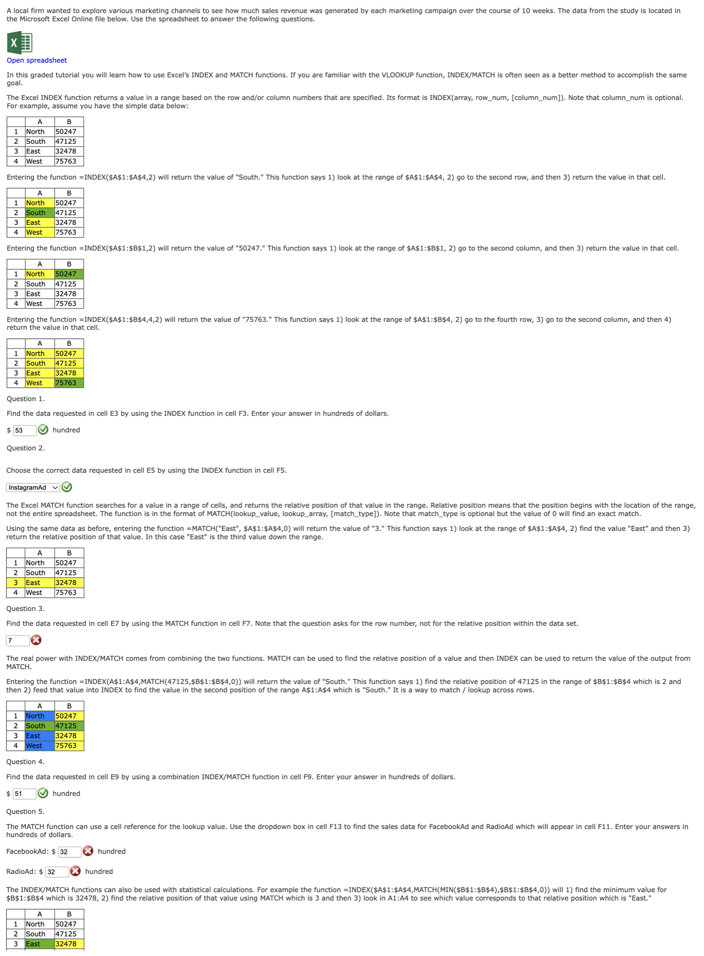
A local firm wanted to explore various marketing channels to see how much sales revenue was generated by each marketing campaign over the course of 10 weeks. The data from the study is located in the Microsoft Excel Online file below. Use the spreadsheet to answer the following questions. Open spreadsheet In this graded tutorial you will learn how to use Excel's INDEX and MATCH functions. If you are familiar with the VLOOKUP function, INDEX/MATCH is often seen as a better method to accomplish the same goal. The Excel INDEX function returns a value in a range based on the row and/or column numbers that are specified. Its format is INDEX(array, row_num, [column_num]). Note that column_num is optional. For example, assume you have the simple data below: A B 1 North 50247 2 South 47125 3 East 32478 4 West 75763 Entering the function =INDEX($A$1:$A$4,2) will return the value of "South." This function says 1) look at the range of $A$1:$A$4, 2) go to the second row, and then 3) return the value in that cell. A North B 1 50247 2 South 47125 3 East 32478 75763 4 West Entering the function =INDEX($A$1:$B$1,2) will return the value of "50247." This function says 1) look at the range of $A$1:$B$1, 2) go to the second column, and then 3) return the value in that cell. 1 A North 2 South 3 East 4 West B 50247 47125 32478 75763 Entering the function =INDEX($A$1:$B$4,4,2) will return the value of "75763." This function says 1) look at the range of $A$1:$B$4, 2) go to the fourth row, 3) go to the second column, and then 4) return the value in that cell. A B 1 North 50247 2 South 47125 3 East 32478 4 West 75763 Question 1. Find the data requested in cell E3 by using the INDEX function in cell F3. Enter your answer in hundreds of dollars. $ 53 Question 2. hundred Choose the correct data requested in cell E5 by using the INDEX function in cell F5. InstagramAdv The Excel MATCH function searches for a value in a range of cells, and returns the relative position of that value in the range. Relative position means that the position begins with the location of the range, not the entire spreadsheet. The function is in the format of MATCH(lookup_value, lookup_array, [match_type]). Note that match_type is optional but the value of 0 will find an exact match. Using the same data as before, entering the function =MATCH("East", $A$1:$A$4,0) will return the value of "3." This function says 1) look at the range of $A$1:$A$4, 2) find the value "East" and then 3) return the relative position of that value. In this case "East" is the third value down the range. A B 50247 1 North 2 South 47125 3 East 4 West Question 3. 32478 75763 Find the data requested in cell E7 by using the MATCH function in cell F7. Note that the question asks for the row number, not for the relative position within the data set. 7 The real power with INDEX/MATCH comes from combining the two functions. MATCH can be used to find the relative position of a value and then INDEX can be used to return the value of the output from MATCH. Entering the function =INDEX(A$1:A$4,MATCH(47125,$B$1:$B$4,0)) will return the value of "South." This function says 1) find the relative position of 47125 in the range of $B$1:$B$4 which is 2 and then 2) feed that value into INDEX to find the value in the second position of the range A$1:A$4 which is "South." It is a way to match/lookup across rows. 1 A North B 50247 2 South 47125 3 East 32478 4 West Question 4. 75763 Find the data requested in cell E9 by using a combination INDEX/MATCH function in cell F9. Enter your answer in hundreds of dollars. $ 51 Question 5. hundred The MATCH function can use a cell reference for the lookup value. Use the dropdown box in cell F13 to find the sales data for FacebookAd and RadioAd which will appear in cell F11. Enter your answers in hundreds of dollars. FacebookAd: $ 32 RadioAd: $ 32 hundred hundred The INDEX/MATCH functions can also be used with statistical calculations. For example the function =INDEX($A$1:$A$4,MATCH(MIN($B$1:$B$4),$B$1:$B$4,0)) will 1) find the minimum value for $B$1:$B$4 which is 32478, 2) find the relative position of that value using MATCH which is 3 and then 3) look in A1:A4 to see which value corresponds to that relative position which is "East." 1 A B North 50247 2 South 47125 3 East 32478