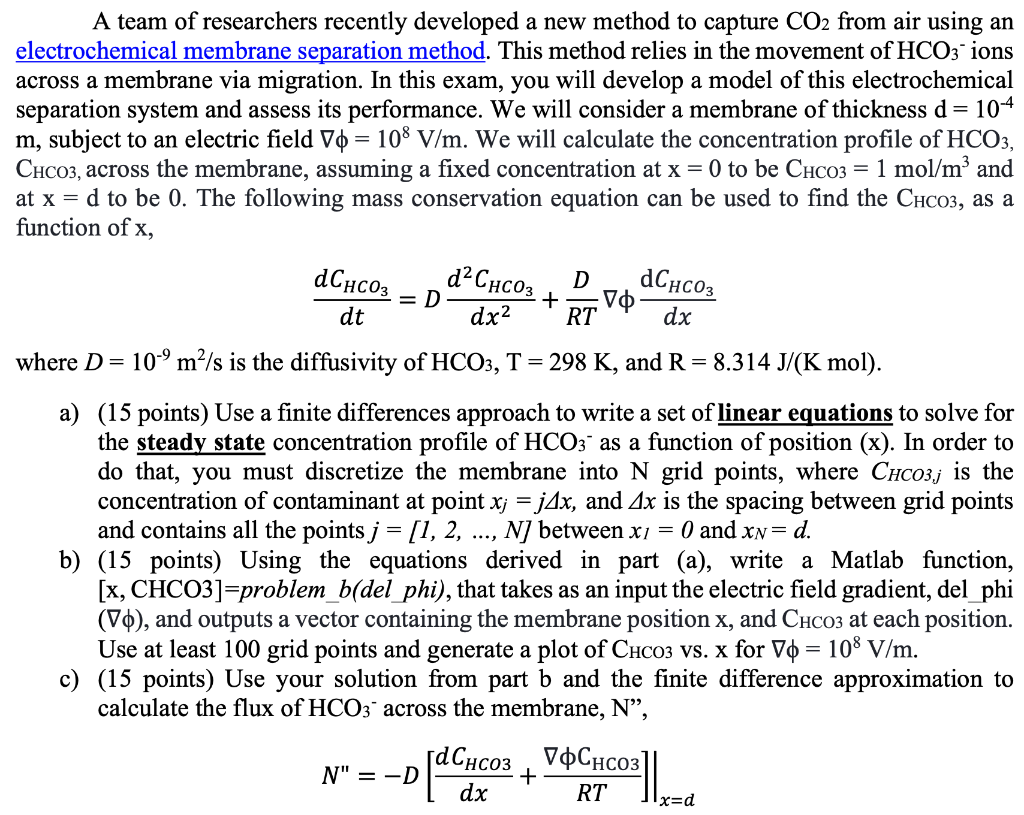
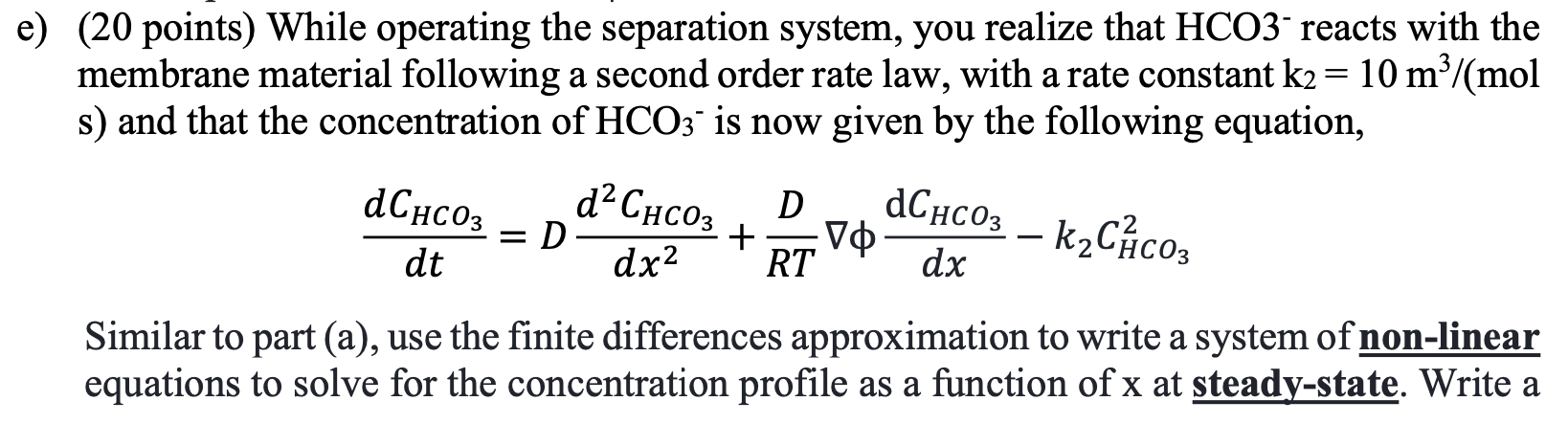
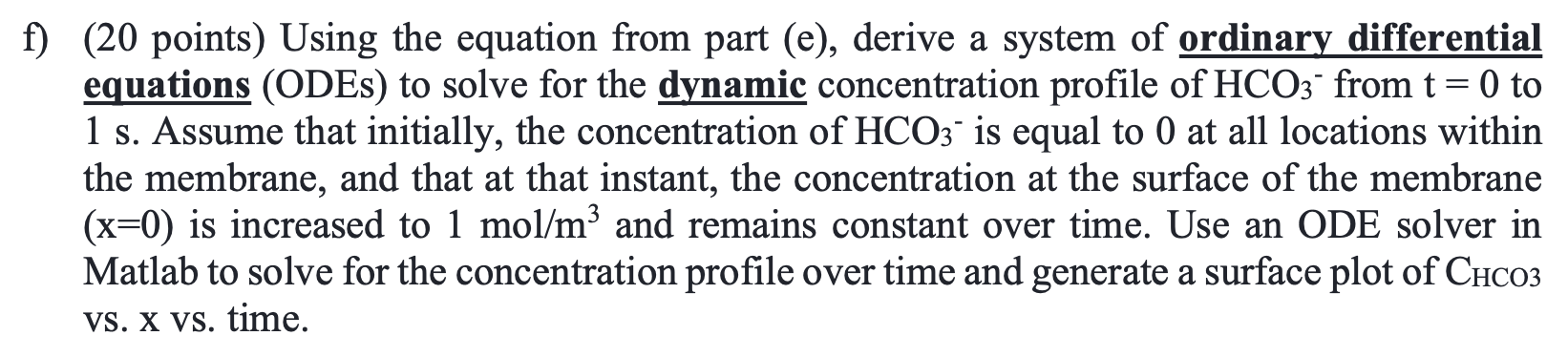
A team of researchers recently developed a new method to capture CO2 from air using an electrochemical membrane separation method. This method relies in the movement of HCO3 ions across a membrane via migration. In this exam, you will develop a model of this electrochemical separation system and assess its performance. We will consider a membrane of thickness d = 104 m, subject to an electric field V0 = 108 V/m. We will calculate the concentration profile of HCO3, CHCO3, across the membrane, assuming a fixed concentration at x = 0 to be CHCO3 = 1 mol/m and at x = d to be 0. The following mass conservation equation can be used to find the CHCO3, as a function of x, - dChcoz dCHCO3 =D dC D + V RT dt dx2 dx where D= 10-9m/s is the diffusivity of HCO3, T = 298 K, and R = 8.314 J/(K mol). a) (15 points) Use a finite differences approach to write a set of linear equations to solve for the steady state concentration profile of HCO3 as a function of position (x). In order to do that, you must discretize the membrane into N grid points, where CHC03,j is the concentration of contaminant at point x; = j4x, and Ax is the spacing between grid points and contains all the points j = [1, 2, ..., N) between x = 0 and xn= d. b) (15 points) Using the equations derived in part (a), write a Matlab function, [x, CHCO3]=problem_b(del_phi), that takes as an input the electric field gradient, del_phi (10), and outputs a vector containing the membrane position x, and CHCO3 at each position. Use at least 100 grid points and generate a plot of CHCO3 Vs. x for V = 108 V/m. c) (15 points) Use your solution from part b and the finite difference approximation to calculate the flux of HCO3 across the membrane, N, , V N" = -D dx RT + x=d d) (15 points) Using your solution from part (b), solve for the concentration profile at 100 different electric fields from Vo = 107 to 109 V/m. Use the surf function to generate a surface plot of CHCO3 vs. x vs. Vo. e) (20 points) While operating the separation system, you realize that HCO3 reacts with the membrane material following a second order rate law, with a rate constant k2 = 10 m3/(mol s) and that the concentration of HCO3 is now given by the following equation, a = > dCHCO3 , dt dCHC03 k2C\cos : D D + VO RT dx2 dx Similar to part (a), use the finite differences approximation to write a system of non-linear equations to solve for the concentration profile as a function of x at steady-state. Write a Matlab function to solve this system of equations and generate a plot of CHCO3 vs. x for Vo = 108 V/m. f) (20 points) Using the equation from part (e), derive a system of ordinary differential equations (ODEs) to solve for the dynamic concentration profile of HCO3 from t = 0 to 1 s. Assume that initially, the concentration of HCO3 is equal to 0 at all locations within the membrane, and that at that instant, the concentration at the surface of the membrane (x=0) is increased to 1 mol/m and remains constant over time. Use an ODE solver in Matlab to solve for the concentration profile over time and generate a surface plot of CHCO3 VS. X vs. time. A team of researchers recently developed a new method to capture CO2 from air using an electrochemical membrane separation method. This method relies in the movement of HCO3 ions across a membrane via migration. In this exam, you will develop a model of this electrochemical separation system and assess its performance. We will consider a membrane of thickness d = 104 m, subject to an electric field V0 = 108 V/m. We will calculate the concentration profile of HCO3, CHCO3, across the membrane, assuming a fixed concentration at x = 0 to be CHCO3 = 1 mol/m and at x = d to be 0. The following mass conservation equation can be used to find the CHCO3, as a function of x, - dChcoz dCHCO3 =D dC D + V RT dt dx2 dx where D= 10-9m/s is the diffusivity of HCO3, T = 298 K, and R = 8.314 J/(K mol). a) (15 points) Use a finite differences approach to write a set of linear equations to solve for the steady state concentration profile of HCO3 as a function of position (x). In order to do that, you must discretize the membrane into N grid points, where CHC03,j is the concentration of contaminant at point x; = j4x, and Ax is the spacing between grid points and contains all the points j = [1, 2, ..., N) between x = 0 and xn= d. b) (15 points) Using the equations derived in part (a), write a Matlab function, [x, CHCO3]=problem_b(del_phi), that takes as an input the electric field gradient, del_phi (10), and outputs a vector containing the membrane position x, and CHCO3 at each position. Use at least 100 grid points and generate a plot of CHCO3 Vs. x for V = 108 V/m. c) (15 points) Use your solution from part b and the finite difference approximation to calculate the flux of HCO3 across the membrane, N, , V N" = -D dx RT + x=d d) (15 points) Using your solution from part (b), solve for the concentration profile at 100 different electric fields from Vo = 107 to 109 V/m. Use the surf function to generate a surface plot of CHCO3 vs. x vs. Vo. e) (20 points) While operating the separation system, you realize that HCO3 reacts with the membrane material following a second order rate law, with a rate constant k2 = 10 m3/(mol s) and that the concentration of HCO3 is now given by the following equation, a = > dCHCO3 , dt dCHC03 k2C\cos : D D + VO RT dx2 dx Similar to part (a), use the finite differences approximation to write a system of non-linear equations to solve for the concentration profile as a function of x at steady-state. Write a Matlab function to solve this system of equations and generate a plot of CHCO3 vs. x for Vo = 108 V/m. f) (20 points) Using the equation from part (e), derive a system of ordinary differential equations (ODEs) to solve for the dynamic concentration profile of HCO3 from t = 0 to 1 s. Assume that initially, the concentration of HCO3 is equal to 0 at all locations within the membrane, and that at that instant, the concentration at the surface of the membrane (x=0) is increased to 1 mol/m and remains constant over time. Use an ODE solver in Matlab to solve for the concentration profile over time and generate a surface plot of CHCO3 VS. X vs. time