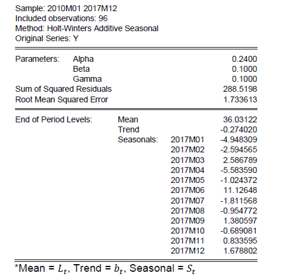
a) The following table gives the estimation results of Holt-Winters Additive Seasonal model. Y denotes the monthly series of new passenger vehicle sales in Australia (in thousands of units). Compute forecast values for January and February of 2018 (97 and 98).

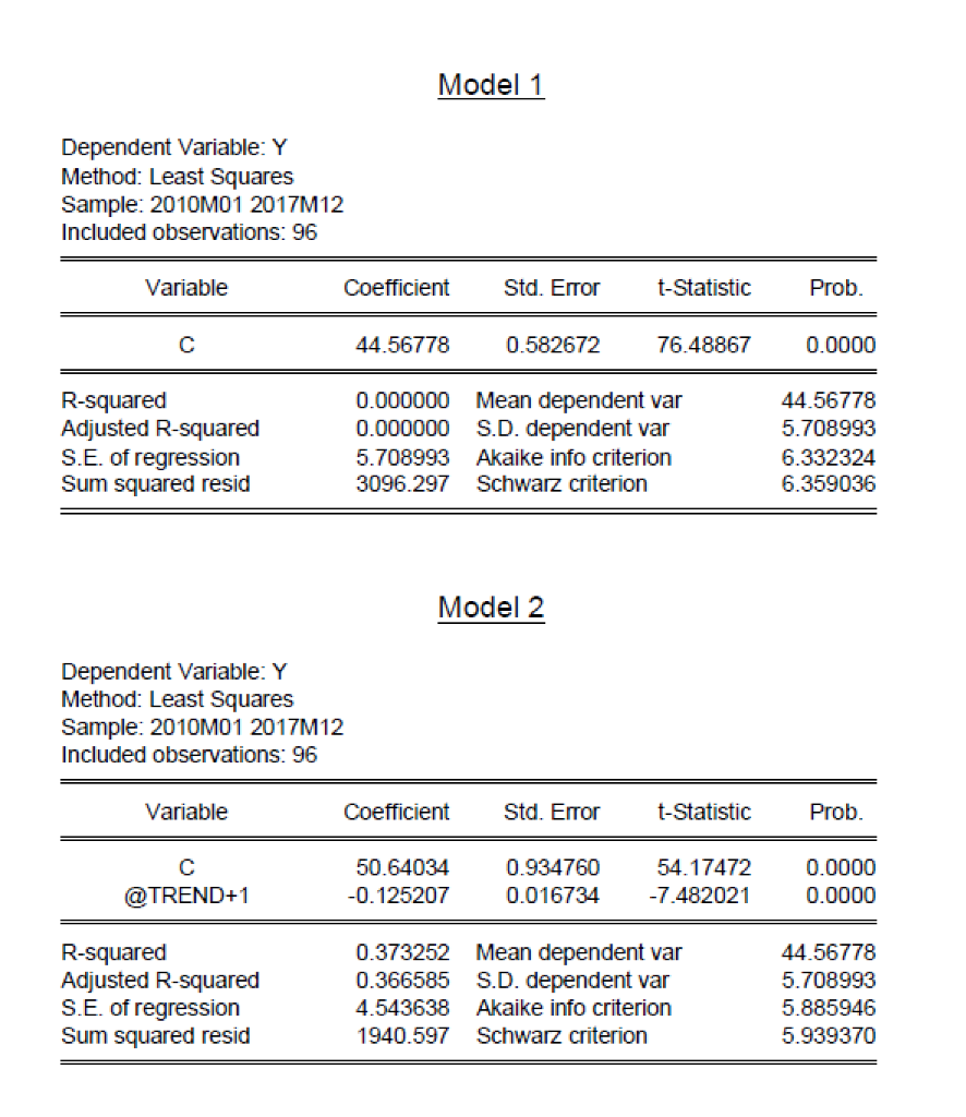
b) The following tables give the estimation results of three regression models. Y denotes the monthly series of new passenger vehicle sales in Australia (in thousands of units). C is an intercept and @TREND+1 represents time trend (@TREND+1 = 1, 2, 3, , 96). @MONTHs are seasonal dummies where @MONTH=1 is equal to 1 for January and 0 otherwise, and @MONTH=2, @MONTH=3, @MONTH=4, @MONTH=5, @MONTH=6, @MONTH=7, @MONTH=8, @MONTH=9, @MONTH=10, and @MONTH=11 are similarly defined for February, March until November, respectively.

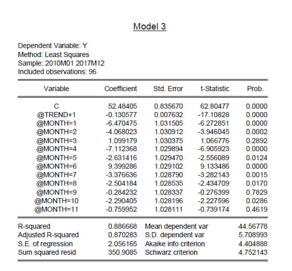
i) Based on Model 3, interpret the estimated coefficients of @TREND+1. ii) Based on Model 3, determine the estimated seasonal factors for January and June. iii) By assuming that all estimated models are adequate, perform a hypothesis testing to determine if there is seasonal variation in the series. iv) Based on the finding in (b)(iii), compute the forecast of new passenger vehicle sales in February 2018. v) Compare forecasts of new passenger vehicle sales in February 2018 calculated in (a) and (b)(iii) and determine which method produced better forecast. [Given that the actual value of new passenger vehicle sales in February 2018 is equal to 33.167 thousand units].

Sample: 2010M01 2017M12 Included observations: 96 Method: Holt-Winters Additive Seasonal Original Series: Y Parameters: Alpha Beta Gamma Sum of Squared Residuals Root Mean Squared Error 0.2400 0.1000 0.1000 288.5198 1.733613 End of Period Levels: Mean Trend Seasonals: 36.03122 -0.274020 -4.948309 -2.594565 2017M01 2017M02 2017M03 2017M04 2017M05 2017M06 2.586789 -5.583590 -1.024372 11.12648 2017M07 2017M08 2017M09 2017M10 2017M11 2017M12 -1.811568 -0.954772 1.380597 -0.689081 0.833595 1.678802 *Mean = Lt. Trend = bt, Seasonal = St Model 1 Dependent Variable: Y Method: Least Squares Sample: 2010M01 2017M12 Included observations: 96 Variable Coefficient Std. Error t-Statistic Prob. 44.56778 0.582672 76.48867 0.0000 0.000000 0.000000 44.56778 5.708993 R-squared Adjusted R-squared S.E. of regression Sum squared resid Mean dependent var S.D. dependent var Akaike info criterion Schwarz criterion 5.708993 3096.297 6.332324 6.359036 Model 2 Dependent Variable: Y Method: Least Squares Sample: 2010M01 2017M12 Included observations: 96 Variable Coefficient Std. Error t-Statistic Prob. @TREND+1 50.64034 -0.125207 0.934760 0.016734 54.17472 -7.482021 0.0000 0.0000 44.56778 R-squared Adjusted R-squared S.E. of regression Sum squared resid 0.373252 Mean dependent var 0.366585 S.D. dependent var 4.543638 Akaike info criterion 1940.597 Schwarz criterion 5.708993 5.885946 5.939370 Model 3 Dependent Variable: Y Method: Least Squares Sample: 2010M01 2017M12 Included observations: 96 Variable Coefficient Std. Error t-Statistic Prob. 52.48405 -0.130577 -6.470475 -4.068023 0.835670 0.007632 1.031505 1.030912 62.80477 -17.10828 -6.272851 -3.946045 0.0000 0.0000 0.0000 0.0002 1.099179 -7.112368 1.030375 1.029894 1.066776 -6.905923 0.2892 0.0000 @TREND+1 @MONTH=1 @MONTH=2 @MONTH=3 @MONTH=4 @MONTH=5 @MONTH=6 @MONTH=7 @MONTH=8 @MONTH=9 @MONTH=10 @MONTH=11 -2.631416 9.399286 -3.376636 -2.504184 1.029470 1.029102 1.028790 1.028535 1.028337 1.028196 1.028111 -2.556089 9.133486 -3.282143 -2.434709 0.0124 0.0000 0.0015 0.0170 -0.284232 -2.290405 -0.759952 -0.276399 -2.227596 -0.739174 0.7829 0.0286 0.4619 44.56778 5.708993 R-squared Adjusted R-squared S.E. of regression Sum squared resid 0.886668 Mean dependent var 0.870283 S.D. dependent var 2.056165 Akaike info criterion 350.9085 Schwarz criterion 4.404888 4.752143 Sample: 2010M01 2017M12 Included observations: 96 Method: Holt-Winters Additive Seasonal Original Series: Y Parameters: Alpha Beta Gamma Sum of Squared Residuals Root Mean Squared Error 0.2400 0.1000 0.1000 288.5198 1.733613 End of Period Levels: Mean Trend Seasonals: 36.03122 -0.274020 -4.948309 -2.594565 2017M01 2017M02 2017M03 2017M04 2017M05 2017M06 2.586789 -5.583590 -1.024372 11.12648 2017M07 2017M08 2017M09 2017M10 2017M11 2017M12 -1.811568 -0.954772 1.380597 -0.689081 0.833595 1.678802 *Mean = Lt. Trend = bt, Seasonal = St Model 1 Dependent Variable: Y Method: Least Squares Sample: 2010M01 2017M12 Included observations: 96 Variable Coefficient Std. Error t-Statistic Prob. 44.56778 0.582672 76.48867 0.0000 0.000000 0.000000 44.56778 5.708993 R-squared Adjusted R-squared S.E. of regression Sum squared resid Mean dependent var S.D. dependent var Akaike info criterion Schwarz criterion 5.708993 3096.297 6.332324 6.359036 Model 2 Dependent Variable: Y Method: Least Squares Sample: 2010M01 2017M12 Included observations: 96 Variable Coefficient Std. Error t-Statistic Prob. @TREND+1 50.64034 -0.125207 0.934760 0.016734 54.17472 -7.482021 0.0000 0.0000 44.56778 R-squared Adjusted R-squared S.E. of regression Sum squared resid 0.373252 Mean dependent var 0.366585 S.D. dependent var 4.543638 Akaike info criterion 1940.597 Schwarz criterion 5.708993 5.885946 5.939370 Model 3 Dependent Variable: Y Method: Least Squares Sample: 2010M01 2017M12 Included observations: 96 Variable Coefficient Std. Error t-Statistic Prob. 52.48405 -0.130577 -6.470475 -4.068023 0.835670 0.007632 1.031505 1.030912 62.80477 -17.10828 -6.272851 -3.946045 0.0000 0.0000 0.0000 0.0002 1.099179 -7.112368 1.030375 1.029894 1.066776 -6.905923 0.2892 0.0000 @TREND+1 @MONTH=1 @MONTH=2 @MONTH=3 @MONTH=4 @MONTH=5 @MONTH=6 @MONTH=7 @MONTH=8 @MONTH=9 @MONTH=10 @MONTH=11 -2.631416 9.399286 -3.376636 -2.504184 1.029470 1.029102 1.028790 1.028535 1.028337 1.028196 1.028111 -2.556089 9.133486 -3.282143 -2.434709 0.0124 0.0000 0.0015 0.0170 -0.284232 -2.290405 -0.759952 -0.276399 -2.227596 -0.739174 0.7829 0.0286 0.4619 44.56778 5.708993 R-squared Adjusted R-squared S.E. of regression Sum squared resid 0.886668 Mean dependent var 0.870283 S.D. dependent var 2.056165 Akaike info criterion 350.9085 Schwarz criterion 4.404888 4.752143