AIM:

Analyze continuous and discrete systems, using MATLAB PC and Example 1.7, 1.8, 1.9, 1.10, and 1.11, pages 37, 38, 39, and 40 of Chapter 1, Sections 1.4 and 1.5, of the guide text, to expand the concepts of continuous modeling and discreet.

DESCRIPTION:

Develop a MATLAB script that meets the objective, taking the exercises proposed in the following pages.

DELIVERY FORMAT:

m file made with MATLAB Editor, or a mlx file made with Live Editor.

Example 1.7

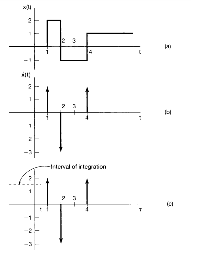
Consider the discontinuous signal x(t) depicted in Figure 1.40(a). Because of the relationship between the continuous-time unit impulse and unit step, we can readily calculate and graph the derivative of this signal. Specifically, the derivative of x(t) is clearly 0, except at the discontinuities. In the case of the unit step, we have seen [eq. (1.72)] that differentiation gives rise to a unit impulse located at the point of discontinuity. Furthermore, by multiplying both sides of eq. (1.72) by any number k, we see that the derivative of a unit step with a discontinuity of size k gives rise to an impulse of area k at the point of discontinuity. This rule also holds for any other signal with a jump discontinuity, such as x(t) in Figure 1.40(a). Consequently, we can sketch its derivative x(t), as in Figure 1.40(b), where an impulse is placed at each discontinuity of x(t), with area equal to the size of the discontinuity. Note, for example, that the discontinuity in x(t) at t = 2 has a value of- 3, so that an impulse scaled by -3 is located at t = 2 in the signal x(t).

Figure 1.40 (a) The discontinuous signal x(t) analyzed in Example 1.7; (b) its derivative x(t); (c) depiction of the recovery of x(t) as the running integral of x(t), illustrated for a value of t between 0 and 1.

As a check of our result, we can verify that we can recover x(t) from x(t). Specifically, since x(t) and x(t) are both zero fort :::::: 0, we need only check that fort > 0,

1.77

As illustrated in Figure 1.40(c), fort 4, all three impulses are within the integration interval, so that the integral equals the sum of all three areas-that is, 2 - 3 + 2 = + 1. The result is exactly the signal x(t) depicted in Figure 1.40(a).

Example 1.8

Consider the RC circuit depicted in Figure 1.1. If we regard vs(t) as the input signal and vc(t) as the output signal, then we can use simple circuit analysis to derive an equation describing the relationship between the input and output. Specifically, from Ohm's law, the current i(t) through the resistor is proportional (with proportionality constant 11 R) to the voltage drop across the resistor; i.e.,

1.80

Similarly, using the defining constitutive relation for a capacitor, we can relate i(t) to the rate of change with time of the voltage across the capacitor:

1.81

Equating the right-hand sides of eqs. (1.80) and (1.81), we obtain a differential equation describing the relationship between the input vs(t) and the output vc(t):

1.82

Example 1.9

Consider Figure 1.2, in which we regard the force f(t) as the input and the velocity v(t) as the output. If we let m denote the mass of the automobile and mpv the resistance due to friction, then equating acceleration-i.e., the time derivative of velocity-with net force divided by mass, we obtain

1.83

i.e.,

1.84

Examining and comparing eqs. (1.82) and (1.84) in the above examples, we see that the input-output relationships captured in these two equations for these two very different physical systems are basically the same. In particular, they are both examples of first-order linear differential equations of the form

1.85

where x(t) is the input, y(t) is the output, and a and bare constants. This is one very simple example of the fact that, by developing methods for analyzing general classes of systems such as that represented by eq. (1.85), we will be able to use them in a wide variety of applications.

Example 1. 1 0

As a simple example of a discrete-time system, consider a simple model for the balance in a bank account from month to month. Specifically, let y[n] denote the balance at the end of the nth month, and suppose that y[n] evolves from month to month according to the equation

1.86

or equivalently,

1.87

where x[n] represents the net deposit (i.e., deposits minus withdrawals) during the nth month and the term 1.01y[n- 1] models the fact that we accrue 1% interest each month.

Example 1. 11

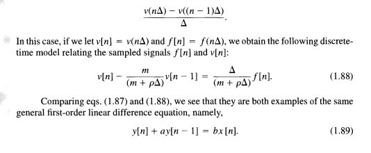
As a second example, consider a simple digital simulation of the differential equation in eq. (1.84) in which we resolve time into discrete intervals oflength and approximate dv(t)ldt at t = n by the first backward difference, i.e.,

As the preceding examples suggest, the mathematical descriptions of systems from a wide variety of applications frequently have a great deal in common, and it is this fact that provides considerable motivation for the development of broadly applicable tools for signal and system analysis. The key to doing this successfully is identifying classes of systems that have two important characteristics: ( 1) The systems in this class have properties and structures that we can exploit to gain insight into their behavior and to develop effective tools for their analysis~ and (2) many systems of practical importance can be accurately modeled using systems in this class. It is on the first of these characteristics that most of this book focuses, as we develop tools for a particular class of systems referred to as linear, time-invariant systems. In the next section, we will introduce the properties that characterize this class, as well as a number of other very important basic system properties. The second characteristic mentioned in the preceding paragraph is of obvious importance for any system analysis technique to be of value in practice. It is a well-established fact that a wide range of physical systems (including those in Examples 1.8-1.10) can be well modeled within the class of systems on which we focus in this book. However, a critical point is that any model used in describing or analyzing a physical system represents an idealization of that system, and thus, any resulting analysis is only as good as the model itself. For example, the simple linear model of a resistor in eq. (1.80) and that of a capacitor in eq. ( 1.81) are idealizations. However, these idealizations are quite accurate for real resistors and capacitors in many applications, and thus, analyses employing such idealizations provide useful results and conclusions, as long as the voltages and currents remain within the operating conditions under which these simple linear models are valid. Similarly, the use of a linear retarding force to represent frictional effects in eq. (1.83) is an approximation with a range of validity. Consequently, although we will not address this issue in the book, it is important to remember that an essential component of engineering practice in using the methods we develop here consists of identifying the range of validity of the assumptions that have gone into a model and ensuring that any analysis or design based on that model does not violate those assumptions.

(b) x(t)=0tx()d i(t)=Rvs(t)vc(t) i(t)=Cdtdvc(t) dtdvc(t)+RC1vc(t)=RC1vs(t) dtdv(t)=m1[f(t)v(t)] dtdv(t)+mv(t)=m1f(t) dtdy(t)+ay(t)=bx(t) y[n]=1.01y[n1]+x[n]. y[n]1.01y[n1]=x[n] v(n)v((n1)) In this case, if we let v[n]=v(n) and f[n]=f(n), we obtain the following discretetime model relating the sampled signals f[n] and v[n] : v[n](m+)mv[n1]=(m+)f[n]. Comparing eqs. (1.87) and (1.88), we see that they are both examples of the same general first-order linear difference equation, namely, y[n]+ay[n1]=bx[n]