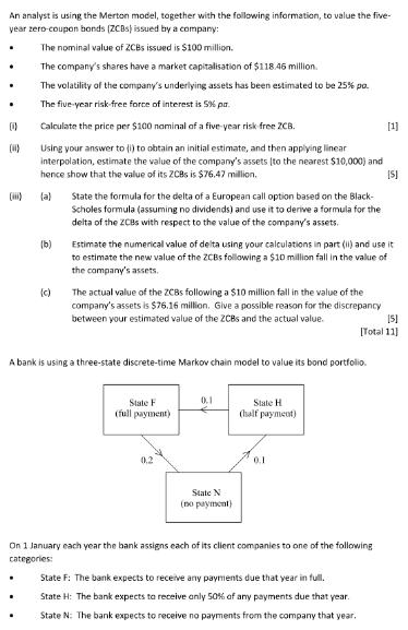
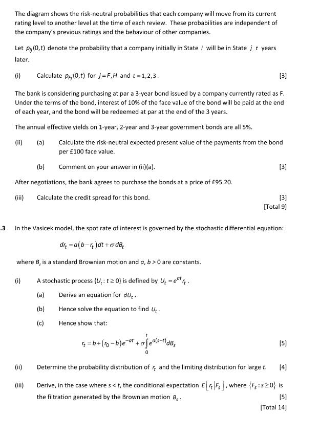
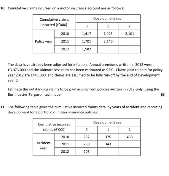
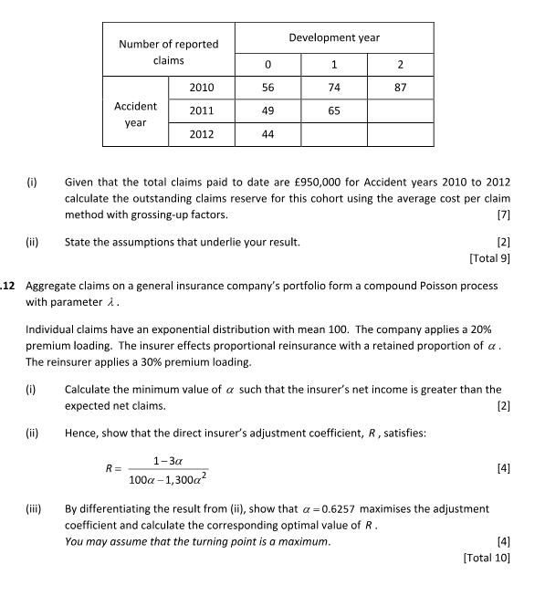
An analyst is using the Merton model, together with the following information, to value the five- year zero-coupon bonds (ZCBS) issued by a company: The nominal value of ZCBs issued is $100 million. The company's shares have a market capitalisation of $118.46 million. The volatility of the company's underlying assets has been estimated to be 25% po. The five-year risk-free force of interest is 5% pa. Calculate the price per $100 nominal of a five-year risk-free ZCB. Using your answer to (i) to obtain an initial estimate, and then applying linear interpolation, estimate the value of the company's assets [to the nearest $10,000) and hence show that the value of its ZCBs is $76.47 million. [5] . . (00) (b) (c) State the formula for the delta of a European call option based on the Black- Scholes formula (assuming no dividends) and use it to derive a formula for the delta of the ZCBs with respect to the value of the company's assets. Estimate the numerical value of delta using your calculations in part (ii) and use it to estimate the new value of the ZCBs following a $10 million fall in the value of the company's assets. The actual value of the ZCBs following a $10 million fall in the value of the company's assets is $76.16 million. Give a possible reason for the discrepancy between your estimated value of the ZCBS and the actual value. A bank is using a three-state discrete-time Markov chain model to value its bond portfolio. State F (full payment) 0.2 0.1 State N (no payment) State H (half payment) 0.1 [5] [Total 11] [1] On 1 January each year the bank assigns each of its client companies to one of the following categories: State F: The bank expects to receive any payments due that year in full. State H: The bank expects to receive only 50% of any payments due that year. State N: The bank expects to receive no payments from the company that year. The diagram shows the risk-neutral probabilities that each company will move from its current rating level to another level at the time of each review. These probabilities are independent of the company's previous ratings and the behaviour of other companies. Let pij (0,t) denote the probability that a company initially in State i will be in State j t years later. (i) Calculate pr; (0,t) for j=F,H and t=1,2,3. [3] The bank is considering purchasing at par a 3-year bond issued by a company currently rated as F. Under the terms of the bond, interest of 10% of the face value of the bond will be paid at the end of each year, and the bond will be redeemed at par at the end of the 3 years. The annual effective yields on 1-year, 2-year and 3-year government bonds are all 5%. (ii) (a) Calculate the risk-neutral expected present value of the payments from the bond per 100 face value. (b) Comment on your answer in (ii)(a). After negotiations, the bank agrees to purchase the bonds at a price of 95.20. (iii) Calculate the credit spread for this bond. (i) .3 In the Vasicek model, the spot rate of interest is governed by the stochastic differential equation: dr = a(b-)dt+odB where B, is a standard Brownian motion and a, b>0 are constants. A stochastic process (U: t20) is defined by Ut=eatt. (a) Derive an equation for du.. (b) Hence solve the equation to find U.. Hence show that: (c) (ii) [3] 4=b+(ro-b)e-at +0jels-11dB [3] [Total 9] [5] [4] Determine the probability distribution of and the limiting distribution for large t. Derive, in the case where s < t, the conditional expectation E[F], where (F:s0, is the filtration generated by the Brownian motion B.. [5] [Total 14] 10 Cumulative claims incurred on a motor insurance account are as follows: Development year 1 1,923 2,140 Cumulative claims incurred ('000) Policy year 2010 2011 2012 The data have already been adjusted for inflation. Annual premiums written in 2012 were 3,073,000 and the ultimate loss ratio has been estimated as 92%. Claims paid to date for policy year 2012 are 441,000, and claims are assumed to be fully run-off by the end of Development year 2. 0 1,417 1,701 1,582 Estimate the outstanding claims to be paid arising from policies written in 2012 only, using the Bornhuetter-Ferguson technique. [6] Cumulative incurred claims ('000) Accident year 11 The following table gives the cumulative incurred claims data, by years of accident and reporting development for a portfolio of motor insurance policies: 2010 2011 2012 2,101 0 252 230 208 Development year 1 375 343 2 438 (i) (ii) Number of reported claims Accident year (ii) 2010 2011 2012 0 56 R= 49 44 Development year 1 74 65 2 87 Given that the total claims paid to date are 950,000 for Accident years 2010 to 2012 calculate the outstanding claims reserve for this cohort using the average cost per claim method with grossing-up factors. [7] State the assumptions that underlie your result. 12 Aggregate claims on a general insurance company's portfolio form a compound Poisson process with parameter 1. [2] [Total 9] Individual claims have an exponential distribution with mean 100. The company applies a 20% premium loading. The insurer effects proportional reinsurance with a retained proportion of a. The reinsurer applies a 30% premium loading. (i) Calculate the minimum value of a such that the insurer's net income is greater than the expected net claims. [2] Hence, show that the direct insurer's adjustment coefficient, R, satisfies: 1-3a 100a-1,300a By differentiating the result from (ii), show that a=0.6257 maximises the adjustment coefficient and calculate the corresponding optimal value of R. You may assume that the turning point is a maximum. [4] [4] [Total 10]