Answer in MATLAB code

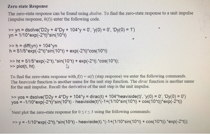
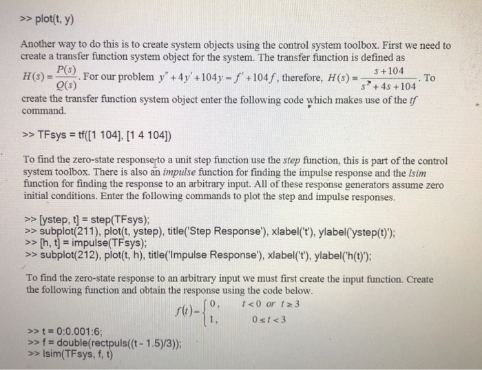
Example given:

s4 with the following input 5.) Find the zero-state response of the system from part 1 for 0 using Isim. 1st > yn dsolve(D2y + 4 Dy +104 y 0', y(0) 0', 'Dy(0) 1) yn 1/10 exp(-2"t)'sin(10t) >>h diff(yn)+ 104 yn h 51/5 exp(-2"t)sin(10t)+ exp(-2"t)"cos(10 t) >>ht 51/5 exp(-2"t).'sin(10t) + exp(-2"t). cos(10 t) >> plot(t, ht) To find the zero-state response with f) u (step response) we enter the following commands The heaviside function is another name for the unit step function. The dirac function is another name for the unit impulse. Recall the derivative of the unit step is the unit impulse. >> yos- dsolve(D2y +4'Dy +104y dirac(t)+ 104'heaviside(t)', y(o)D 0) yos--1/10'exp(-2"t)'sin(10t) - heaviside() (-1+(1/10 sin(10t)+ cos(10 t)) 'exp(-2"t) Next plot the zero-state response for 0 ts3 using the following commands: > y - -1/10 exp(-2") sin(10") heavisidel)/ (61+(1/10'sin(10-) + cos/(10"t)-exp(-2-7): >> plot(t, y) Another way to do this is to create system objects using the control system toolbox. First we need to create a transfer function system object for the system. The transfer function is defined as H(For our problem y+4y+104y-f+104f, therefore, H (s) create the transfer function system object enter the following code which makes use of the tf S +104 +4s +104 0(s) .To command. TFsys tl1 104], [1 4 104]) To find the zero-state response to a unit step function use the step function, this is part of the control system toolbox. There is also an impulse function for finding the impulse response and the lsim function for finding the response to an arbitrary input. All of these response generators assume zero initial conditions. Enter the following commands to plot the step and impulse responses. >> [ystep, t] step(TFsys); >subplot(211), plott, ystep), title('Step Response), xlabel(t), ylabel(ystep()); >> h, t-impulse(TFsys); >> subplot(212), plot(t, h), title('Impulse Response), xlabel('t), ylabel(h()); To find the zero-state response to an arbitrary input we must first create the input function. Create the following function and obtain the response using the code below. 0, 1, tt 0:0.001:6 >s f double(rectpuls(t-1.5y3) >>Isim(TFsys, f, t