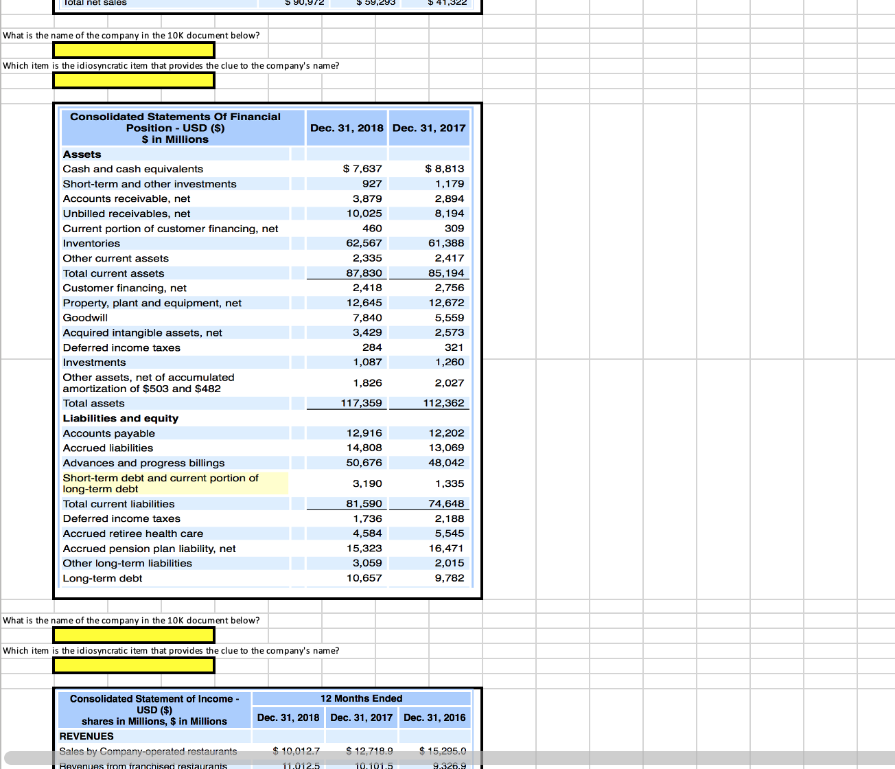
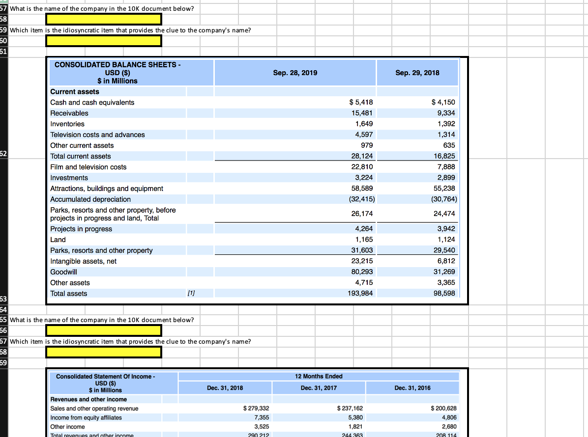
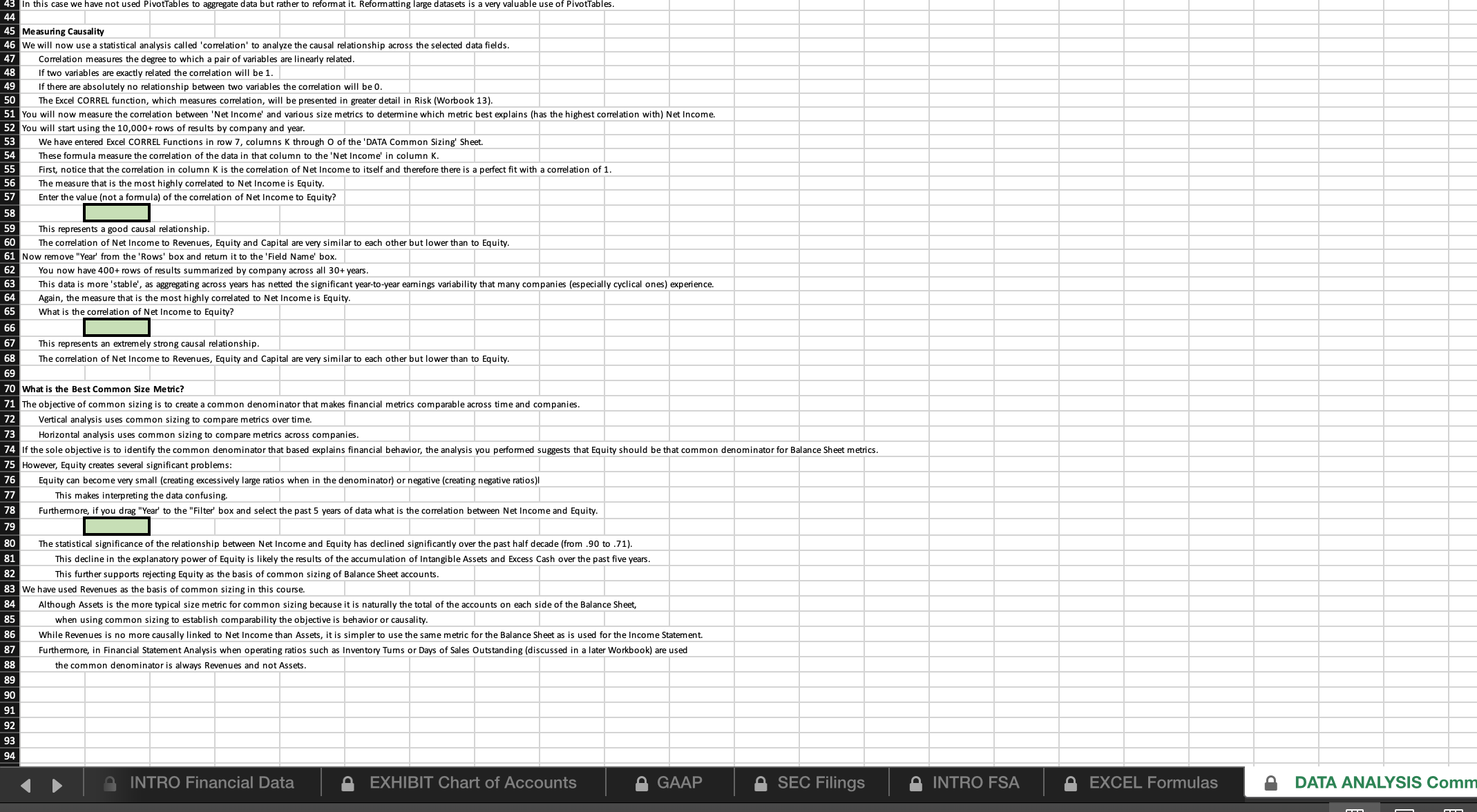
answer it please : https://ccnymailcuny-my.sharepoint.com/:x:/g/personal/malam008_citymail_cuny_edu/Ea6JKeTr8SFHt2qszPDUavcBHxD6zFZUCXvCFivFNs4Kuw?e=h6i4EF

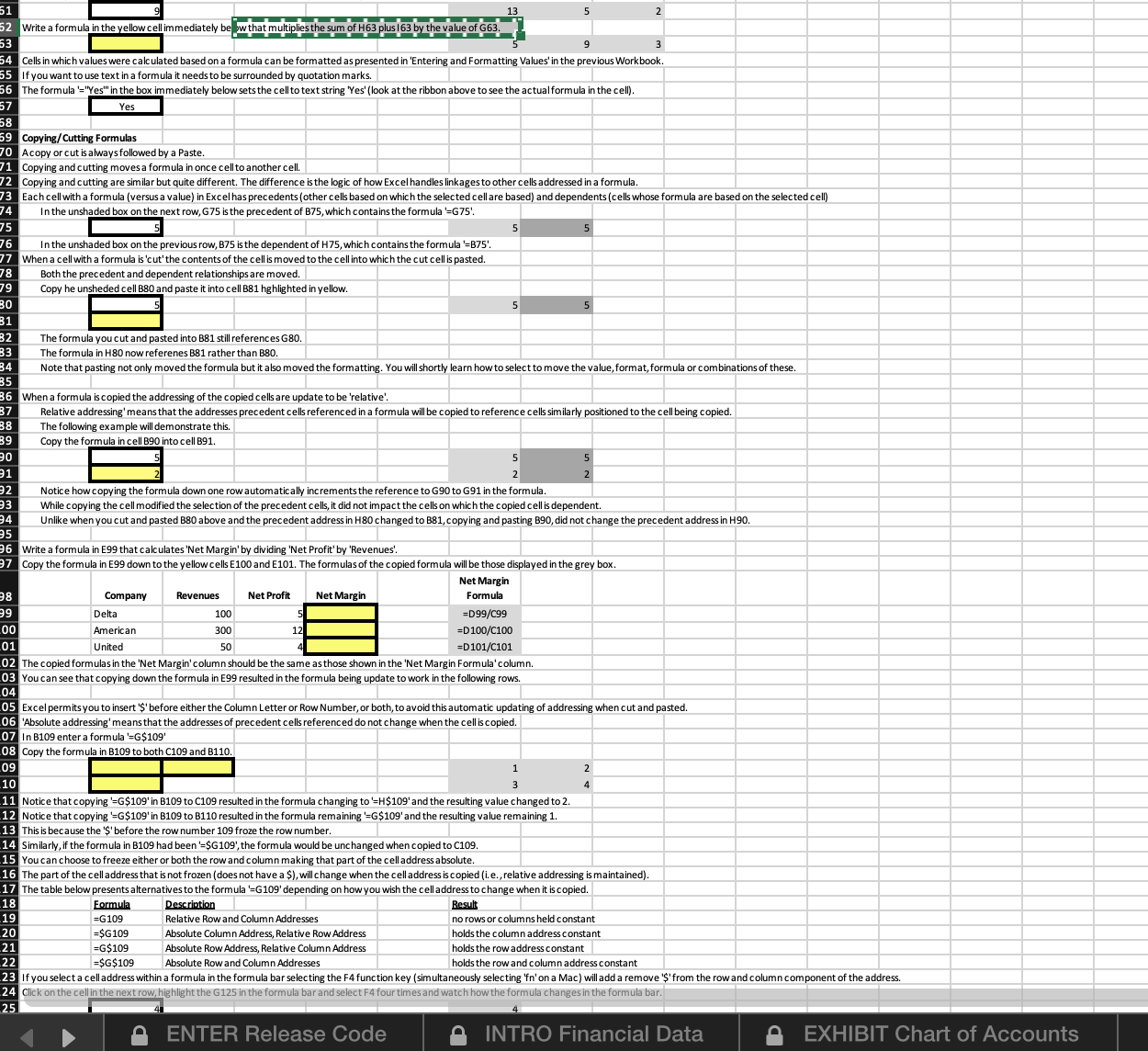
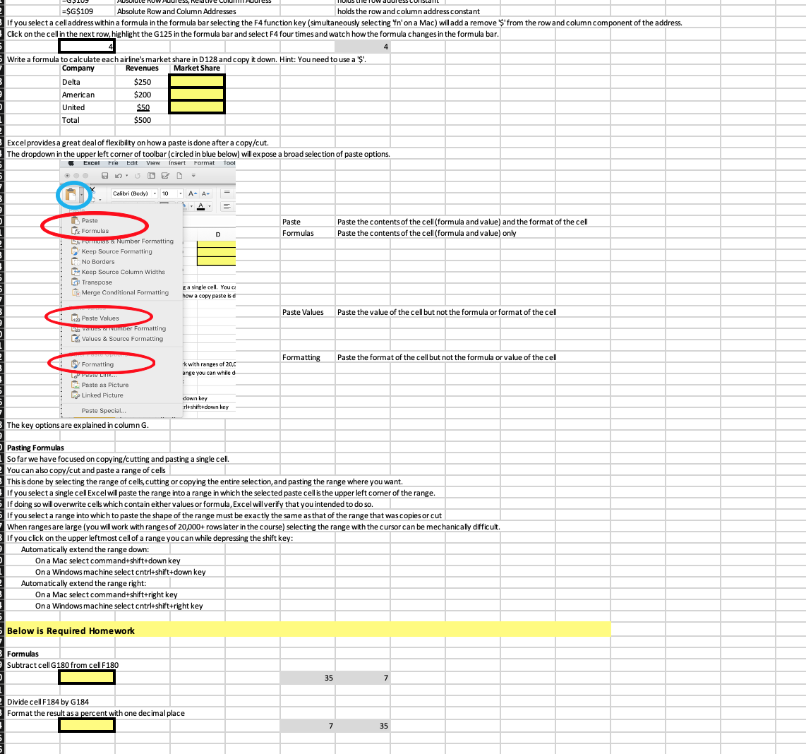
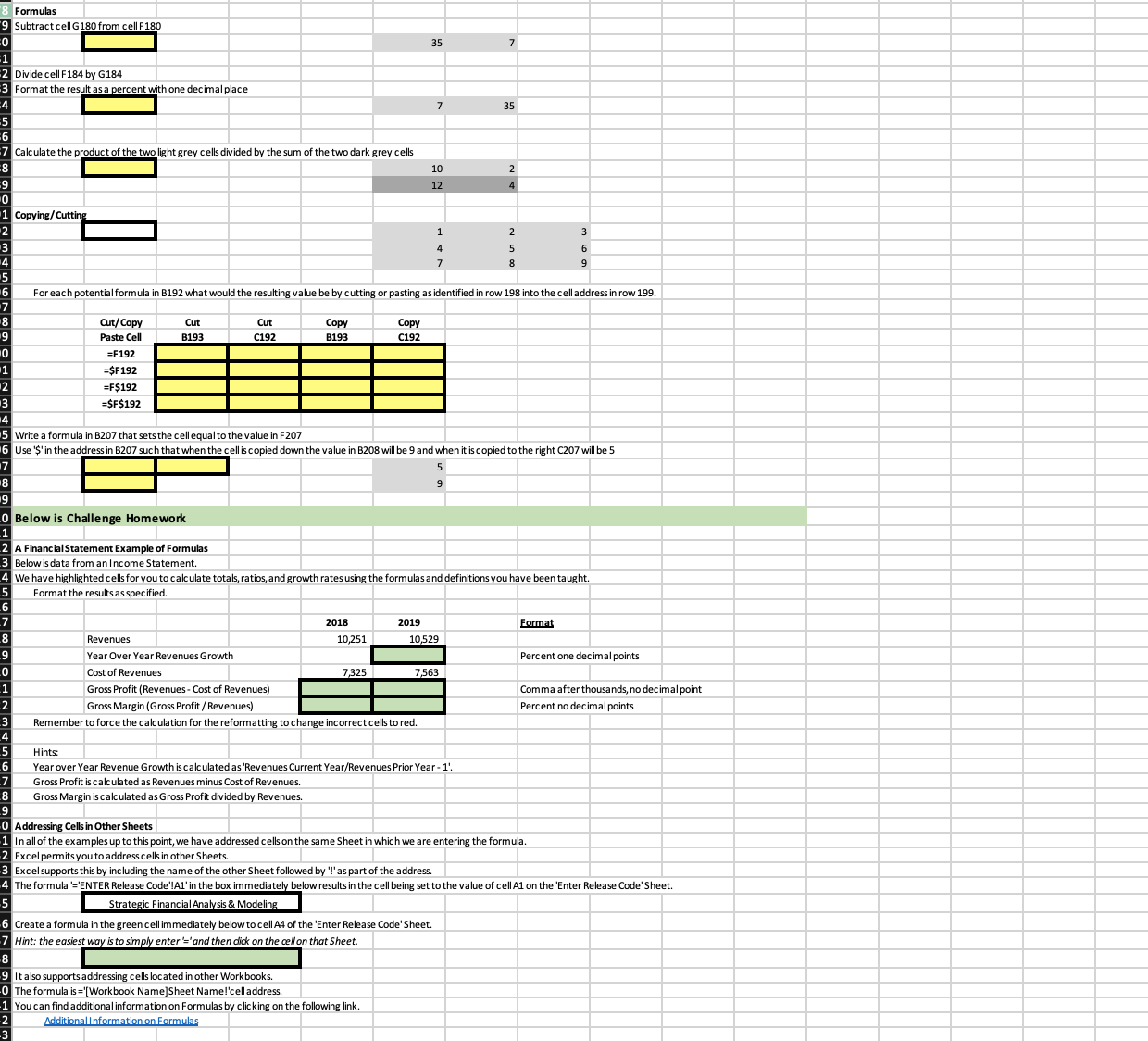
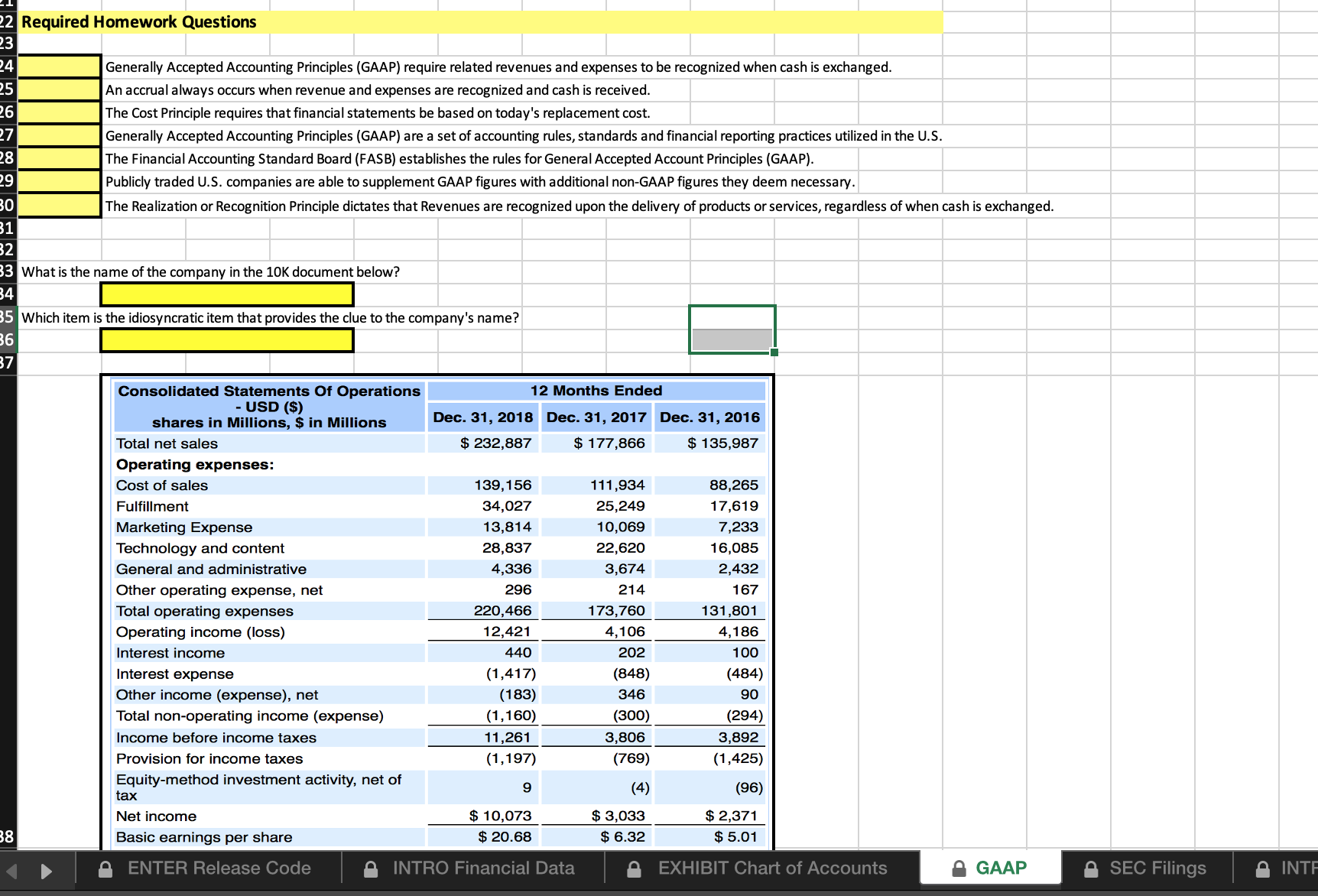
5 Write a formula in the yellow cell immediately be ow that multiplies the sur 13 Cells in which values were calculated based on a formula can be formatted as presented in 'Entering and Formatting Values' in the previous Workbook if you want to use text in a formula it needs to be surrounded by quotation marks. The formula '="Yes" in the box immediately below sets the cell to text string "Yes' (look at the ribbon above to see the actual formula in the cell). Yes Copying/ Cutting Formulas Acopy or cut is always followed by a Paste. Copying and cutting moves a formula in once cell to another cell. Copying and cutting are similar but quite different. The difference is the logic of how Excel handles linkages to other cells addressed in a formula. Each cell with a formula (versus a value) in Excel has precedents ( other cells based on which the selected cell are based) and dependents (cells whose formula are based on the selected cell) In the unshaded box on the next row, G75 is the precedent of B75, which contains the formula '=G75' In the unshaded box on the previous row, B75 is the de ndent of H75, which contains the formula '=875' When a cell with a formula is 'cut' the contents of the cell is moved to the cell into which the cut cell is pasted. Both the precedent and dependent relationships are moved. Copy he unsheded cell B80 and paste it into cell B81 highlighted in yellow. The formula you cut and pasted into B81 still references G80. The formula in H80 now referenes B81 rather than B80. Note that pasting not only moved the formula but it also moved the formatting. You will shortly learn how to select to move the value, format, formula or combinations of these. When a formula is copied the addressing of the copied cells are update to be 'relative' Relative addressing' means that the addresses precedent cells referenced in a formula will be copied to reference cells similarly positioned to the cell being copied. The following example will demonstrate this Copy the formula in cell B90 into cell B91. Notice how copying the formula down one row automatically increments the reference to G90 to G91 in the formula. While copying the cell modified the selection of the precedent cells, it did not impact the cells on which the copied cell is dependent. Unlike when you cut and pasted B80 above and the precedent address in H80 changed to B81, copying and pasting B90, did not change the precedent address in H90. Write a formula in E99 that calculates 'Net Margin' by dividing 'Net Profit' by 'Revenues'. Copy the formula in E99 down to the yellow cells E100 and E101. The formulas of the copied formula will be those displayed in the grey box. Net Margin Company Revenues Net Profit Net Margin Formula Delta 100 =D99/099 American 300 =D100/C100 United 50 =D101/C101 The copied formulas in the 'Net Margin' column should be the same as those shown in the 'Net Margin Formula' column. 04 You can see that copying down the formula in E99 resulted in the formula being update to work in the following rows. )5 Excel permits you to insert'S' before either the Column Letter or Row Number, or both, to avoid this automatic updating of addressing when cut and pasted. 06 'Absolute addressing' means that the addresses of precedent cells referenced do not change when the cell is copied. 07 In B109 enter a formula =G$109' 08 Copy the formula in B109 to both C109 and B1 10. 09 Notice that copying '=G$109' in B109 to C109 resulted in the formula changing to '=H$109' and the resulting value changed to 2. Notice that copying =G$109' in B109 to B1 10 resulted in the formula remaining '=G$109' and the resulting value remaining 1. This is because the 'S' before the row number 109 froze the row number. Similarly, if the formula in B109 had been '=$G109', the formula would be unchanged when copied to C109 You can choose to freeze either or both the row and column making that part of the cell address absolute. The part of the cell address that is not frozen ( does not have a $), will change when the cell address is copied (i. e., relative addressing is maintained). The table below presents alternatives to the formula '=G109' depending on how you wish the cell address to change when it is copied. Formula Description sesul =G 109 Relative Row and Column Addresses no rows or columns held constant SG103 Absolute Column Address, Relative Row Address holds the column address constant =G$109 Absolute Row Address, Relative Column Address holds the row address constant =$G$109 Absolute Row and Column Addresses holds the row and column address constant If you select a cell address within a formula in the formula bar selecting the F4 function key (simultaneously selecting 'n' on a Mac) will add a remove 's' from the row and column component of the address. 24 Click on the cell in the next row, highlight the G125 in the formula bar and select F4 four times and watch how the formula changes in the formula bar. 25 ENTER Release Code INTRO Financial Data A EXHIBIT Chart of Accounts=$G$109 Absolute Row and Column Addresses holds the row and column address constant If you select a cell address within a formula in the formula bar selecting the F4 function key (simultaneously selecting 'n' on a Mac) will add a remove 's' from the row and column component of the address. Click on the cell in the next row, highlight the G125 in the formula bar and select F4 four times and watch how the formula changes in the formula bar. Write a formula to calculate each airline's market share in D 128 and copy it down. Hint: You need to use a 's'. Company Revenues Market Share Delta $250 American $200 United $50 Total $500 Excel provides a great deal of flexibility on how a paste is done after a copy/cut. The dropdown in the upper left corner of toolbar (circled in blue below) will expose a broad selection of paste options. Excel File Edit View Insert Format Tool Calibri (Body) . 10 . A- A b. A - Paste Paste fix Formulas Paste the contents of the cell (formula and value) and the format of the cell commons & Number Formatting Formulas Paste the contents of the cell (formula and value) only Keep Source Formatting LEa No Borders Keep Source Column Widths Ga Transpose Is Merge Conditional Formatting E a single cell. You ca how a copy paste is d Liza Paste Values Paste Values Paste the value of the cell but not the formula or format of the cell ze wanner Formatting in Values & Source Formatting Formatting k with ranges of 20,C Formatting Paste the format of the cell but not the formula or value of the cell ange you can while d Paste as Picture Le Linked Picture dawn key Paste Special. ri+shift+down key The key options are explained in column G. Pasting Formulas So far we have focused on copying/cutting and pasting a single cell You can also copy/cut and paste a range of cells This is done by selecting the range of cells, cutting or copying the entire selection, and pasting the range where you want. if you select a single cell Excel will paste the range into a range in which the selected paste cell is the upper left corner of the range. If doing so will overwrite cells which contain either values or formula, Excel will verify that you intended to do so. you select a range into which to paste the shape of the range must be exactly the same as that of the range that was copies or cut When ranges are large (you will work with ranges of 20,000+ rows later in the course) selecting the range with the cursor can be mechanically difficult. If you click on the upper leftmost cell of a range you can while depressing the shift key: Automatically extend the range down: On a Mac select command+shift+down key On a Windows machine select cntri+ shift+down key Automatically extend the range right: On a Mac select command+shift+right key On a Windows machine select cntri+ shift+right key Below is Required Homework Formulas Subtract cell G180 from cell F180 35 Divide cell F 184 by G184 Format the result as a percent with one decimal place 35Formulas Subtract cell G 180 from cell F 180 35 Divide cell F 184 by G184 Format the result as a percent with one decimal place 35 Calculate the product of the two light grey cells divided by the sum of the two dark grey cells 10 12 N Copying/ Cutting n N For each potential formula in B192 what would the resulting value be by cutting or pasting as identified in row 198 into the cell address in row 199 Cut/ Copy Cut Cut Copy Copy Paste Cell B193 C192 B193 C192 =F192 =$F192 =F$192 =$F$192 Write a formula in B207 that sets the cell equal to the value in F207 Use 'S' in the address in B207 such that when the cell is copied down the value in B208 will be 9 and when it is copied to the right C207 will be 5 Below is Challenge Homework A Financial Statement Example of Formulas Below is data from an Income Statement. We have highlighted cells for you to calculate totals, ratios, and growth rates using the formulas and definitions you have been taught Format the results as specified. 2018 2019 Format Revenues 10,251 10,529 Year Over Year Revenues Growth Percent one decimal points Cost of Revenues 7325 7563 Gross Profit (Revenues - Cost of Revenues) Comma after thousands, no decimal point Gross Margin (Gross Profit / Revenues) Percent no decimal points Remember to force the calculation for the reformatting to change incorrect cells to red Hints: Year over Year Revenue Growth is calculated as 'Revenues Current Year/Revenues Prior Year - 1 Gross Profit is calculated as Revenues minus Cost of Revenues. Gross Margin is calculated as Gross Profit divided by Revenues Addressing Cells in Other Sheets In all of the examples up to this point, we have addressed cells on the same Sheet in which we are entering the formula. Excel permits you to address cells in other Sheets. Excel supports this by including the name of the other Sheet followed by "!' as part of the address. The formula '='ENTER Release Code'!Al' in the box immediately below results in the cell being set to the value of cell Al on the 'Enter Release Code' Sheet. Strategic Financial Analysis & Modeling Create a formula in the green cell immediately below to cell A4 of the 'Enter Release Code' Sheet. Hint: the easiest way is to simply enter '=' and then dick on the cell on that Sheet. It also supports addressing cells located in other Workbooks The formula is ='[Workbook Name]Sheet Name!'cell address. You can find additional information on Formulas by clicking on the following link. Additional Information on FormulasRequired Homework Questions Generally Accepted Accounting Principles (GAAP) require related revenues and expenses to be recognized when cash is exchanged. An accrual always occurs when revenue and expenses are recognized and cash is received. The Cost Principle requires that financial statements be based on today's replacement cost. Generally Accepted Accounting Principles (GAAP) are a set of accounting rules, standards and financial reporting practices utilized in the U.S. The Financial Accounting Standard Board (FASB) establishes the rules for General Accepted Account Principles (GAAP) Publicly traded U.S. companies are able to supplement GAAP figures with additional non-GAAP figures they deem necessary. The Realization or Recognition Principle dictates that Revenues are recognized upon the delivery of products or services, regardless of when cash is exchanged. What is the name of the company in the 10K document below? Which item is the idiosyncratic item that provides the clue to the company's name? Consolidated Statements Of Operations 12 Months Ended - USD ($) shares in Millions, $ in Millions Dec. 31, 2018 Dec. 31, 2017 Dec. 31, 2016 Total net sales $ 232,887 $ 177,866 $ 135,987 Operating expenses: Cost of sales 139, 156 111,934 88,265 Fulfillment 34,027 25,249 17,619 Marketing Expense 13,814 10,069 7,233 Technology and content 28,837 22,620 16,085 General and administrative 4,336 3,674 2,432 Other operating expense, net 296 214 167 Total operating expenses 220,466 173,760 131,801 Operating income (loss) 12,421 4,106 4,186 Interest income 440 202 100 Interest expense (1,417) (848) (484) Other income (expense), net (183) 346 90 Total non-operating income (expense) (1, 160) (300 294) Income before income taxes 11,261 3,806 3,892 Provision for income taxes (1, 197) 769 (1,425) Equity-method investment activity, net of tax (4) (96) Net income $ 10,073 $ 3,033 $ 2,371 Basic earnings per share $ 20.68 $ 6.32 $ 5.01 ENTER Release Code INTRO Financial Data EXHIBIT Chart of Accounts GAAP SEC Filings & INTEWhat is the name of the company in the 10K document below? Which item is the idiosyncratic item that provides the clue to the company's name? Consolidated Statements Of Financial Position - USD ($) Dec. 31, 2018 Dec. 31, 2017 $ in Millions Assets Cash and cash equivalents $ 7,637 $ 8,813 Short-term and other investments 927 1,179 Accounts receivable, net 3,879 2,894 Unbilled receivables, net 10,025 3, 194 Current portion of customer financing, net 460 309 Inventories 62,567 61,388 Other current assets 2,335 2,417 Total current assets 37,830 85, 194 Customer financing, net 2,418 2,756 Property, plant and equipment, net 12,645 12,672 Goodwill 7,840 5,559 Acquired intangible assets, net 3,429 2,573 Deferred income taxes 284 321 Investments 1,087 1,260 Other assets, net of accumulated amortization of $503 and $482 1,826 2,027 Total assets 117,359 112,362 Liabilities and equity Accounts payable 12,916 12,202 Accrued liabilities 14,808 13,069 Advances and progress billings 50,676 48,042 Short-term debt and current portion of long-term deb 3,190 1,335 Total current liabilities 81,590 74,648 Deferred income taxes 1,736 2, 188 Accrued retiree health care 4,584 5,545 Accrued pension plan liability, net 15,323 16,471 Other long-term liabilities 3,059 2,015 Long-term debt 10,657 9,782 What is the name of the company in the 10K document below? Which item is the idiosyncratic item that provides the clue to the company's name? Consolidated Statement of Income - 12 Months Ended USD ($) shares in Millions, $ in Millions Dec. 31, 2018 |Dec. 31, 2017 | Dec. 31, 2016 REVENUES Sales by Company-operated restaurants $ 10,012.7 $ 12,718.9 $ 15,295.07 What is the name of the company in the 10K document below? 58 Which item is the idiosyncratic item that provides the clue to the company's name? CONSOLIDATED BALANCE SHEETS - USD ($) Sep. 28, 2019 Sep. 29, 2018 $ in Millions Current assets Cash and cash equivalents $ 5,418 $ 4,150 Receivables 15,481 9,334 Inventories 1,649 1,392 Television costs and advances 4,597 1,314 Other current assets 979 635 Total current assets 28,124 16,825 Film and television costs 22,810 7,888 Investments 3,224 2,899 Attractions, buildings and equipment 58,589 65,238 Accumulated depreciation (32,415) (30,764) Parks, resorts and other property, before 26,174 24,474 projects in progress and land, Total Projects in progress 4,264 3,942 Land 1,165 1,124 Parks, resorts and other property 31,603 29,540 Intangible assets, net 23,215 6,812 Goodwill 80,293 31,269 Other assets 4,715 3,365 Total assets [1] 193,984 98,598 5 What is the name of the company in the 10K document below? Which item is the idiosyncratic item that provides the clue to the company's name? Consolidated Statement Of Income - 12 Months Ended USD ($) $ in Millions Dec. 31, 2018 Dec. 31, 2017 Dec. 31, 2016 Revenues and other income Sales and other operating revenue $ 279,332 $ 237,162 $ 200,628 Income from equity affiliates 7,355 5,380 4,806 Other income 3,525 1,82 2,680In this case we have not used Reformatting large datasets is a very valuable use of PivotTables. 45 Measuring Causality We will now use a statistical analysis called 'correlation' to analyze the causa the causal relationship across the selected data fields. Correlation measures the degree to which a pair of variables are linearly related 48 if two variables are exactly related the correlation will be 1. if there are absolutely no relationship between two variables the correlation will be 0. The Excel CORREL function, which measures correlation, will be presented in greater detail in Risk (Worbook 13). You will now measure the correlation between 'Net Income' and various size metrics to determine which metric best explains (has the highest correlation with) Net Income. You will start using the 10,000+ rows of results by company and year. We have entered Excel CORREL Functions in row 7, columns K through O of the 'DATA Common Sizing' Sheet. These formula measure the correlation of the data in that column to the 'Net Income' in column K. First, notice that the correlation in column K is the correlation of Net Income to itself and therefore there is a perfect fit with a correlation of 1. The measure that is the most highly correlated to Net Income is Equity. nter the value (not a formula) of the correlation of Net Income to Equity? This represents a good causal relationship. The correlation of Net Income to Revenues, Equity and Capital are very similar to each other but lower than to Equity. Now remove "Year' from the 'Rows' box and return it to the 'Field Name' box. You now have 400+ rows of results summarized by company across all 30+ years. This data is more 'stable', as aggregating across years has netted the significant year-to-year earnings variability that many companies (especially cyclical ones) experience. Again, the measure that is the most highly correlated to Net Income is Equity. What is the correlation of Net Income to Equity? This represents an extremely strong causal relationship. The correlation of Net Income to Revenues, Equity and Capital are very similar to each other but lower than to Equity. 70 What is the Best Common Size Metric? The objective of common sizing is to create a common denominator that makes financial metrics comparable across time and companies. Vertical analysis uses common sizing to compare metrics over time. Horizontal analysis uses common sizing to compare metrics across companies. 74 if the sole objective is to identify the common denominator that based explains financial behavior, the analysis you performed suggests that Equity should be that common denominator for Balance Sheet metrics. However, Equity creates several significant problems: Equity can become very small (creating excessively large ratios when in the denominator) or negative (creating negative ratios) This makes interpreting the data confusing. Furthermore, if you drag "Year' to the "Filter' box and select the past 5 years of data what is the correlation between Net Income and Equity. 80 The statistical significance of the relationship between Net Income and Equity has declined significantly over the past half decade (from .90 to .71). 81 Re S This decline in the explanatory power of Equity is likely the results of the accumulation of Intangible Assets and Excess Cash over the past five years. This further supports rejecting Equity as the basis of common sizing of Balance Sheet accounts 83 We have used Revenues as the basis of common sizing in this course Although Assets is the more typical size metric for common sizing because it is naturally the total of the accounts on each side of the Balance Sheet, when using common sizing to establish comparability the objective is behavior or causality. 87 While Revenues is no more causally linked to Net Income than Assets, it is simpler to use the same metric for the Balance Sheet as is used for the Income Statement. 8 8 Furthermore, in Financial Statement Analysis when operating ratios such as Inventory Tums or Days of Sales Outstanding (discussed in a later Workbook) are used the common denominator is always Revenues and not Assets. 92 93 94 INTRO Financial Data EXHIBIT Chart of Accounts A GAAP A SEC Filings & INTRO FSA A EXCEL Formulas DATA ANALYSIS Comm