Answer Q # 1,2,3,4
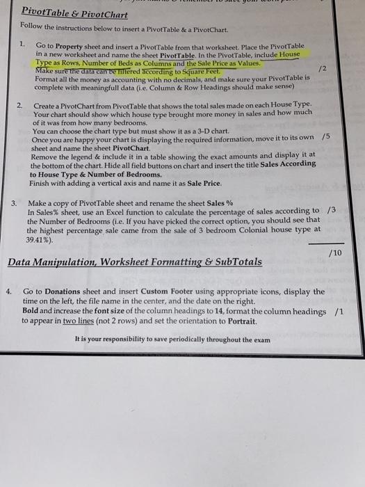
PivotTable & PivotChart Follow the instructions below to insert a PivotTable & a PivotChart. 1. Go to Property sheet and insert a PivotTable from that worksheet. Place the PivotTable in a new worksheet and name the sheet PivotTable. In the Pivot Table, include House Type as Rows, Number of Beds as Columns and the Sale Price as Values Make sure the data can be intered according to Square Feet. Format all the money as accounting with no decimals, and make sure your PivotTable is complete with meaningfull data (ie. Column & Row Headings should make sense) /2 2. Create a PivotChart from Pivottable that shows the total sales made on each House Type. Your chart should show which house type brought more money in sales and how much of it was from how many bedrooms. You can choose the chart type but must show it as a 3-D chart Once you are happy your chart is displaying the required information, move it to its own /5 sheet and name the sheet PivotChart. Remove the legend & include it in a table showing the exact amounts and display it at the bottom of the chart. Hide all field buttons on chart and insert the title Sales According to House Type & Number of Bedrooms, Finish with adding a vertical axis and name it as Sale Price. 3. Make a copy of Pivot Table sheet and rename the sheet Sales % In Sales sheet use an Excel function to calculate the percentage of sales according to /3 the Number of Bedrooms (i.e. If you have picked the correct option, you should see that the highest percentage sale came from the sale of 3 bedroom Colonial house type at 39.41%). /10 Data Manipulation, Worksheet Formatting & SubTotals 4. Go to Donations sheet and insert Custom Footer using appropriate icons, display the time on the left, the file name in the center, and the date on the right. Bold and increase the font size of the column headings to 14, format the column headings /1 to appear in two lines (not 2 rows) and set the orientation to Portrait. It is your responsibility to save periodically throughout the exam PivotTable & PivotChart Follow the instructions below to insert a PivotTable & a PivotChart. 1. Go to Property sheet and insert a PivotTable from that worksheet. Place the PivotTable in a new worksheet and name the sheet PivotTable. In the Pivot Table, include House Type as Rows, Number of Beds as Columns and the Sale Price as Values Make sure the data can be intered according to Square Feet. Format all the money as accounting with no decimals, and make sure your PivotTable is complete with meaningfull data (ie. Column & Row Headings should make sense) /2 2. Create a PivotChart from Pivottable that shows the total sales made on each House Type. Your chart should show which house type brought more money in sales and how much of it was from how many bedrooms. You can choose the chart type but must show it as a 3-D chart Once you are happy your chart is displaying the required information, move it to its own /5 sheet and name the sheet PivotChart. Remove the legend & include it in a table showing the exact amounts and display it at the bottom of the chart. Hide all field buttons on chart and insert the title Sales According to House Type & Number of Bedrooms, Finish with adding a vertical axis and name it as Sale Price. 3. Make a copy of Pivot Table sheet and rename the sheet Sales % In Sales sheet use an Excel function to calculate the percentage of sales according to /3 the Number of Bedrooms (i.e. If you have picked the correct option, you should see that the highest percentage sale came from the sale of 3 bedroom Colonial house type at 39.41%). /10 Data Manipulation, Worksheet Formatting & SubTotals 4. Go to Donations sheet and insert Custom Footer using appropriate icons, display the time on the left, the file name in the center, and the date on the right. Bold and increase the font size of the column headings to 14, format the column headings /1 to appear in two lines (not 2 rows) and set the orientation to Portrait. It is your responsibility to save periodically throughout the exam
 Answer Q # 1,2,3,4


