Answer the following using the R statistical computing platform. Please should include the code you wrote plus the output of such code and English rhetoric / coding comments where necessary.

Question

Using the "accept-reject" algorithm, generate observations from the binomial distribution as target distribution and the uniform distribution as proposal distribution. Reverse the roles and carry out the same simulation and note the differences.

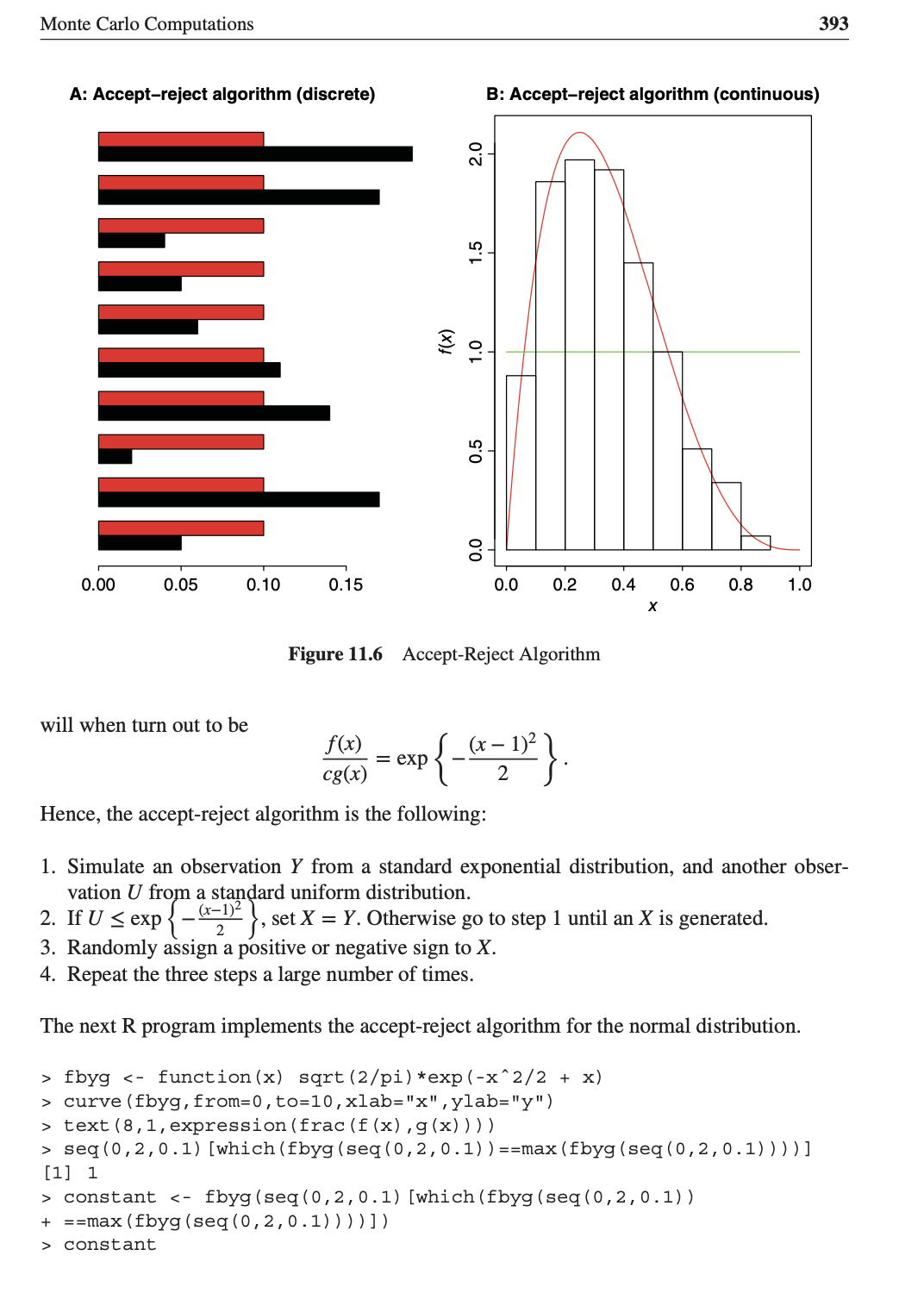
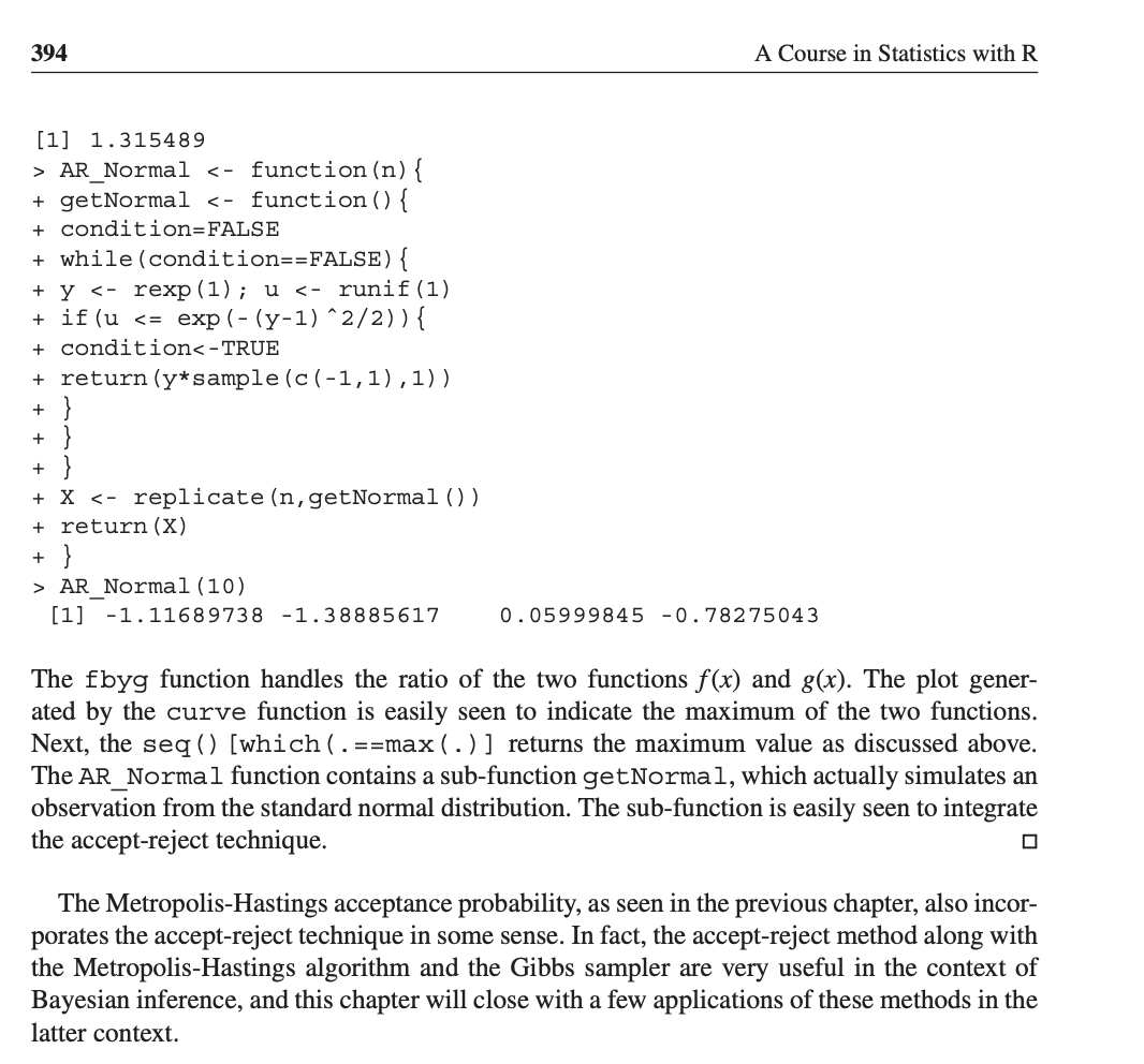
11.5 The Accept-Reject Technique Direct simulation from probability distribution F will turn out to be an inefficient technique in many cases, and in a handful of cases it is simply not possible to do so. This forces us to simulate observations from a different distribution and then find a technique to transfer those observations to the distribution of interest through an appropriate way. First, simulation from discrete distributions will be considered. Suppose that X is an RV of interest with pmf {p;, j 2 0}, and as such simulation from {p; } is a difficult task. Assume that an efficient technique is available to simulate observations of an RV Y with pmf {q;, j 2 0}. It is important that X and Y have the same range. The accept-reject technique then accepts the simulated values of Y for X with a probability proportional to Px / qy. That is, the simulated values of Y are accepted with certain probabilities. Let c be a constant such that "i 0. qi (11.2) The accept-reject algorithm for discrete RVs is then given in the following steps: 1. Simulate an observation Y with pmf { q;, j 2 0}. 2. Generate an observation from U(0, 1), say U. 3. Set X = Y if U q prob AR_Demo AR Demo (p_prob , q_prob , 100) [1] 10 9 3 10 10 6 [27] 1 5 4 9 10 2 [53] 4 9 10 9 8 9 4 [79] 10 10 10 5 2 1 > round (table (AR_Demo (p_prob, q_prob , 10000) ) /10000, 2) 1 2 3 4 5 6 7 8 9 10 0. 05 0. 18 0. 02 0. 14 0. 11 0. 06 0. 05 0. 04 0. 16 0. 19 > barplot (rbind (p_prob, q prob) , horiz TRUE, col=1 : 2, beside=TRUE, + main="A: Accept-Reject Algorithm (Discrete) ") The function AR_Demo has been named for the program of the accept-reject technique. The steps of the technique can be easily seen as integrated in the AR_Demo function. Note that the proportions of the simulated observations for X are closer to the required probability, see Part A of Figure 11.6. The accept-reject technique is now extended to the case of continuous RVs. As with the discrete case, let Y be the proposal RV with pdf g(x) and X denote the target RV with pdf f(x). Assume that the following condition holds true: f(v) 8(v) SC, Vy. The accept-reject algorithm for continuous RVs is then given in the following steps: 1. Simulate an observation Y with pdf g. 2. Generate an observation from U(0, 1), say U. 3. Set X = Y if U fbyg text (8 , 1, expression (frac (f (x) , g (x) ) ) ) > seq (0, 2, 0.1) [which (fbyg (seq (0 , 2, 0.1) ) ==max (fbyg (seg (0, 2, 0.1) ) ) ) ] [1] 1 constant constant394 A Course in Statistics with R [1] 1. 315489 > AR Normal AR Normal (10) [1] -1. 11689738 -1.38885617 0 . 05999845 -0. 78275043 The fbyg function handles the ratio of the two functions f(x) and g(x). The plot gener- ated by the curve function is easily seen to indicate the maximum of the two functions. Next, the seq () [which ( . ==max ( . ) ] returns the maximum value as discussed above. The AR_Normal function contains a sub-function getNormal, which actually simulates an observation from the standard normal distribution. The sub-function is easily seen to integrate the accept-reject technique. The Metropolis-Hastings acceptance probability, as seen in the previous chapter, also incor- porates the accept-reject technique in some sense. In fact, the accept-reject method along with the Metropolis-Hastings algorithm and the Gibbs sampler are very useful in the context of Bayesian inference, and this chapter will close with a few applications of these methods in the latter context