Answering questions with graphical analysis and (graphical) data support?explanation for each curve shift and for the reasonableness of your depiction of where the economy is at each point with respect to the price pressure and the output gap

Be sure to provide full explanation/support for each of the curve shifts and the corresponding short-run SRAS-AD equilibrium point at each time.

Remember, the short-run equilibrium point is determined by where the economy lands with respect to price pressure (upward, downward, none) and the output gap (negative, positive, none). {While the output gap is captured in the AS-AD model in terms of realized real GDP relative to LRAS, there is a richer set of economic data available to characterize this gap such as unemployment, labor participation, industrial production ... }Be sure to capture what happens to the drivers of SRAS (cost of major intermediate materials, cost of capital, cost of labor, expected future profits...) and to the drivers of AD (C, I, G, NX and what drives each of these components)

Setting: Early Spring 2020 United Sates

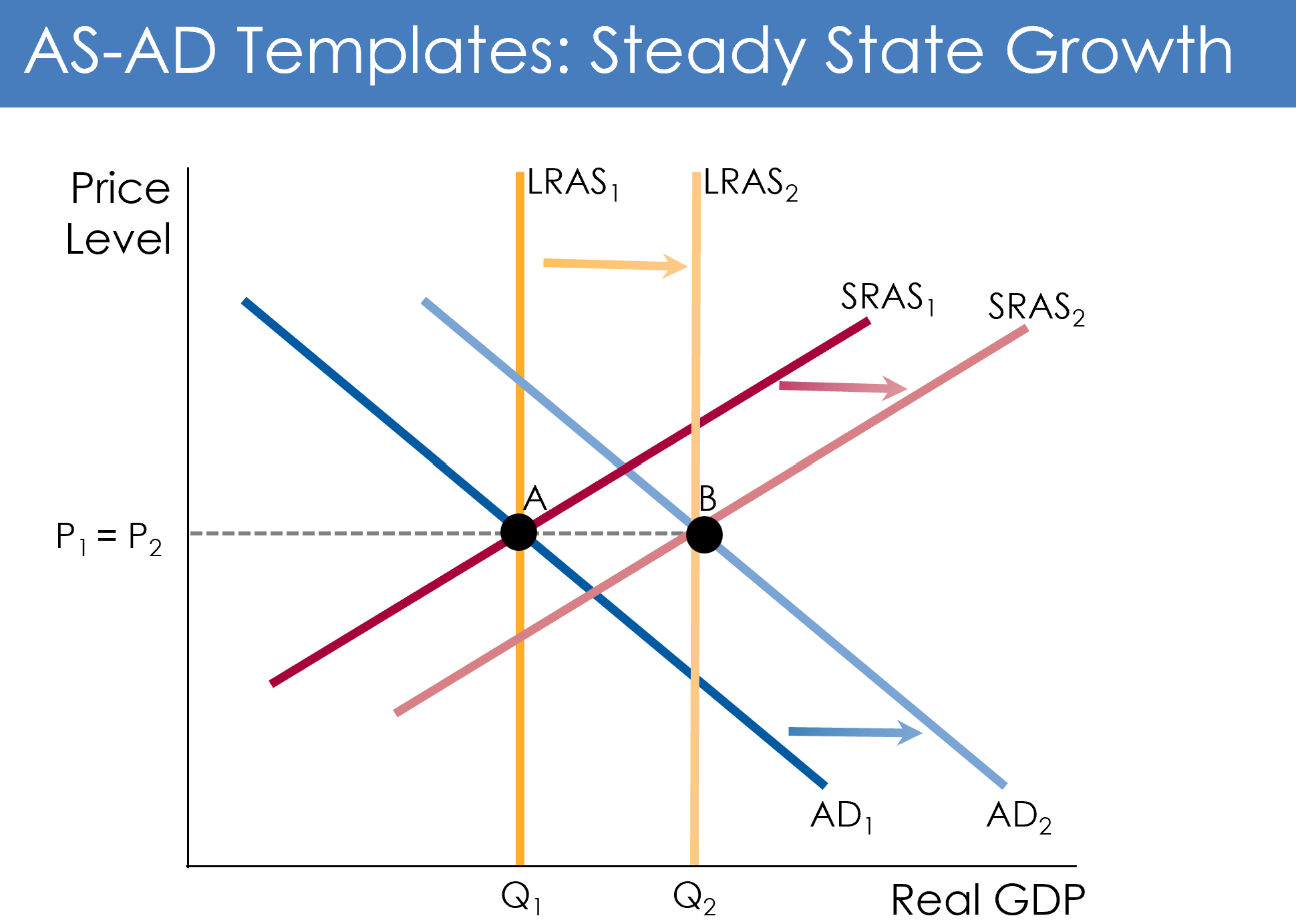
Time 0: The Doldrums

Time 0 (The Doldrums) / Point A: captures where the economy lies before the COVID shock (early 2020)

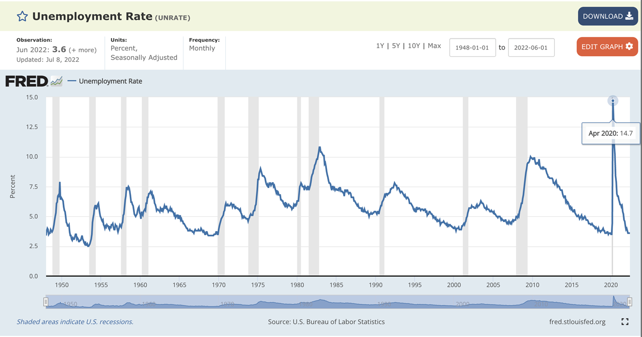
Macroeconomic life in the US is ok but not "booming;" some signs of upward price pressure; unemployment getting closer to "natural" rate but room to go; Fed balance sheet still reflecting quantitative easing; interest rates on the way back down after 3 years of tightening; the Federal deficit was increasing again.

Analysis

a) What does the AS-AD analysis look like for the U.S. in the period before the COVID shock hit? That is, where is Point A on the AS-AD graph?

b) Be sure fully explain why you have modelled Point A (time 0) as you have. Your explanation should address the unemployment, output, and inflation/deflation dynamics at the time as well as considering the components of aggregate demand.

Please use these "event time" definitions as opposed to a strict calendar timeline:

Time 1 to Time 2": Global Pandemic Shock & Response

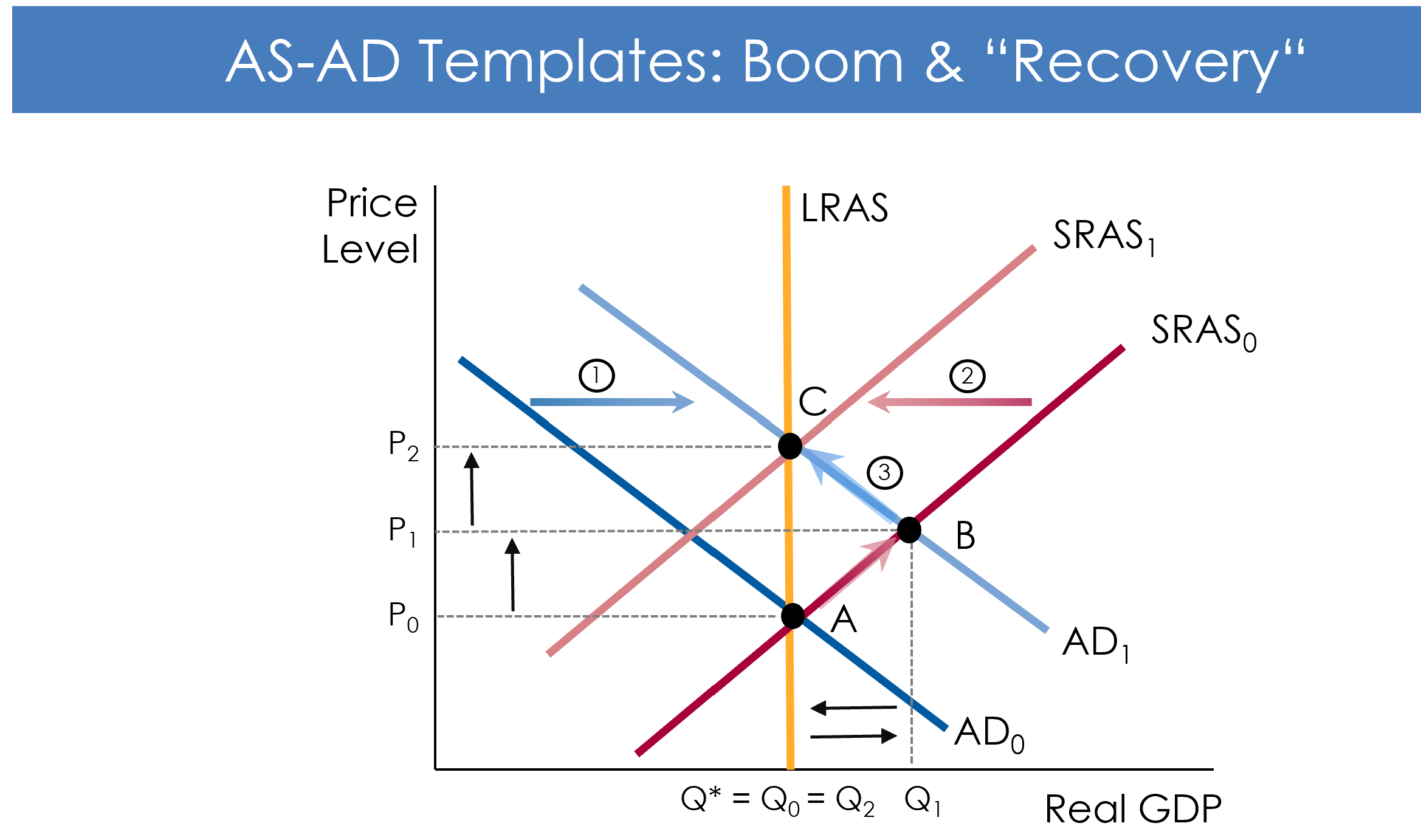
Time 1 / Point B: captures the "immediate" impact of the shock as it "hit" / "rolled over" the economy. In this case, it captures the impact the response of households, firms and the rest of the world to the pandemic as well as the impact of the various governments' public-health oriented regulatory responses (as opposed to the monetary and fiscal responses) (beginning end of March as both voluntary and involuntary lock-downs and "from home" arrangements began impacting the economy)

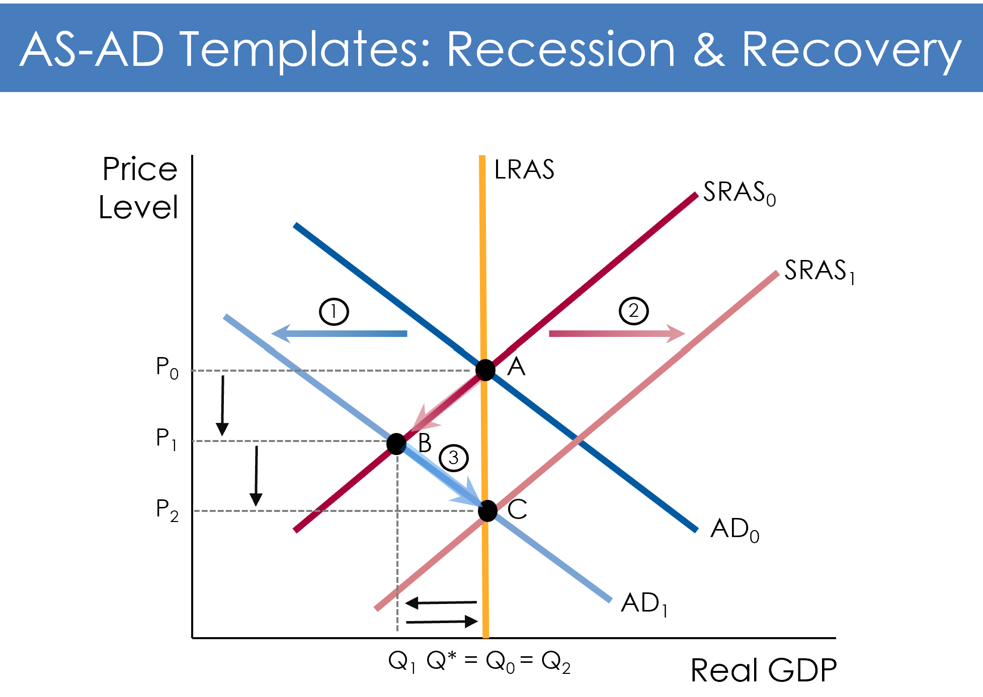
Time 2 / Point C: captures the market adjustment - on its own - over time without macroeconomic policy. (There is no actual calendar time here because it is purely a thought experiment. Conceptually, how would the market adjust on its own with no fiscal (automatic or discretionary) or monetary policy intervention.)

Time 2' / Point D: captures the combination of the market response AND any macroeconomic policy (automatic or discretionary. {Let's artificially set this to be a point in time when the economy was still directly and significantly impacted by COVID but macroeconomic policy had also kicked in. Let's say, roughly, end of 2020, beginning of 2021}

Time 2" / Point E: captures the combination of the market response, the evolution of any macroeconomic policy (automatic or discretionary, AND the evolution of the underlying public health disruption to the economy (i.e. "living with" COVID). {Let's say, roughly, the end of 2021.}

\f\fAS-AD Templates: Boom & "Recovery" Price LRAS SRAS Level SRAS 2 C P 2 3 P 1 B Po A AD ADo Q * = Q = Q2 Q 1 Real GDPUnemployment Rate (UNRATE) DOWNLOAD Observation: Units: Frequency: Jun 2022: 3.6 (+ more) Percent, Monthly 1Y | 5Y | 10Y | Max 1948-01-01 to 2022-06-01 EDIT GRAPH Updated: Jul 8, 2022 Seasonally Adjusted FRED ~- Unemployment Rate 15.0 12.5 Apr 2020: 14.7 10.0 Percent 7.5 5.0 WM 2.5 0.0 1950 1955 1960 1965 1970 1975 1980 1985 1990 1995 2000 2005 2010 2015 2020 41950 2000 Shaded areas indicate U.S. recessions. Source: U.S. Bureau of Labor Statistics fred.stlouisfed.org