Answers as soon as possible pleasee & thank youu!!

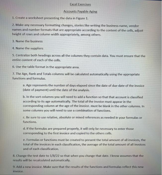
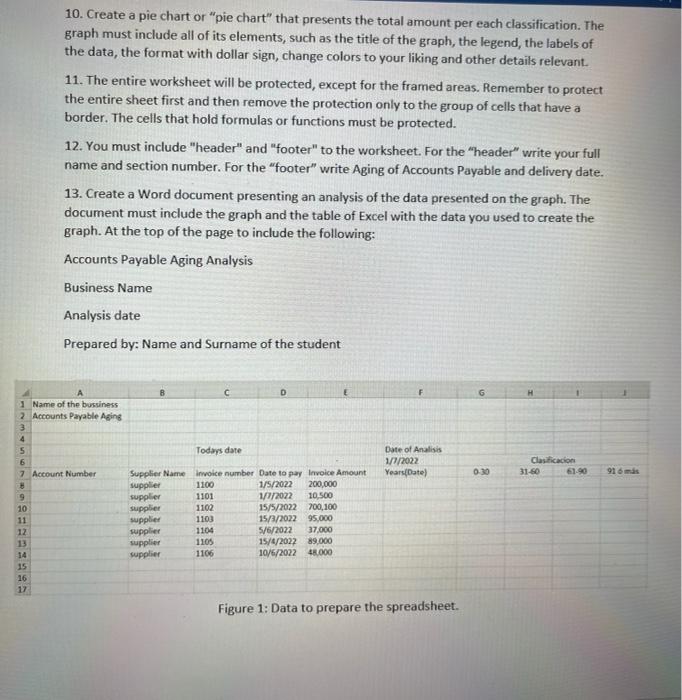
Excel Exercises Accounts Payable Aging 1. Create a worksheet presenting the data in Figure 1. 2. Make any necessary formatting changes, stories like writing the business name, vendor names and number formats that are appropriate according to the content of the cells, adjust height of rows and column width appropriately, among others. 3. Name the business 4. Name the suppliers 5. Centralize both headings across all the columns they contain data. You must ensure that the entire content of each of the cells. 6. Use the table format in the appropriate area. 7. The Age, Rank and Totals columns will be calculated automatically using the appropriate functions and formulas. a. Age represents the number of days elapsed since the date of due date of the invoice (date of payment) until the date of the analysis. b. In the sort columns you will need to add a function so that that account is classified according to its age automatically. The total of the invoice must appear in the corresponding column at the age of the invoice. must be blank in the other columns. In some columns you will need to use a combination of functions. c. Be sure to use relative, absolute or mixed references as needed in your formulas or functions. d. If the formulas are prepared properly, it will only be necessary to enter those corresponding to the first invoice and copied to the others cells. e. Formulas or functions must be created to present the total amount of all invoices, the total of the invoices in each classification, the average of the total amount of all invoices and of each classification. 8. Change the test date to 1/8/22 so that when you change that date. I know assumes that the results will be recalculated automatically. 9. Add a new invoice. Make sure that the results of the functions and formulas reflect this new invoice. 10. Create a pie chart or "pie chart" that presents the total amount per each classification. The graph must include all of its elements, such as the title of the graph, the legend, the labels of the data, the format with dollar sign, change colors to your liking and other details relevant. 11. The entire worksheet will be protected, except for the framed areas. Remember to protect the entire sheet first and then remove the protection only to the group of cells that have a border. The cells that hold formulas or functions must be protected. 12. You must include "header" and "footer" to the worksheet. For the "header" write your full name and section number. For the "footer" write Aging of Accounts Payable and delivery date. 13. Create a Word document presenting an analysis of the data presented on the graph. The document must include the graph and the table of Excel with the data you used to create the graph. At the top of the page to include the following: Accounts Payable Aging Analysis Business Name Analysis date Prepared by: Name and Surname of the student Todays date Date of Analisis 1/7/2022 Clasificacion 31-60 Years(Date) Supplier Name invoice number Date to pay Invoice Amount supplier 1100 1/5/2022 200,000 supplier 1101 1/7/2022 10,500 supplier 1102 supplier 1103 15/5/2022 700,100 15/3/2022 95,000 5/6/2022 37,000 15/4/2022 89,000 supplier 1104 supplier 1105 supplier 1106 10/6/2022 48,000 Figure 1: Data to prepare the spreadsheet. 1 Name of the bussiness 2 Accounts Payable Aging 3 4 5 6 7 Account Number B 9 10 11 12 13 14 15 16 17 0:30 61-90 916 ms Excel Exercises Accounts Payable Aging 1. Create a worksheet presenting the data in Figure 1. 2. Make any necessary formatting changes, stories like writing the business name, vendor names and number formats that are appropriate according to the content of the cells, adjust height of rows and column width appropriately, among others. 3. Name the business 4. Name the suppliers 5. Centralize both headings across all the columns they contain data. You must ensure that the entire content of each of the cells. 6. Use the table format in the appropriate area. 7. The Age, Rank and Totals columns will be calculated automatically using the appropriate functions and formulas. a. Age represents the number of days elapsed since the date of due date of the invoice (date of payment) until the date of the analysis. b. In the sort columns you will need to add a function so that that account is classified according to its age automatically. The total of the invoice must appear in the corresponding column at the age of the invoice. must be blank in the other columns. In some columns you will need to use a combination of functions. c. Be sure to use relative, absolute or mixed references as needed in your formulas or functions. d. If the formulas are prepared properly, it will only be necessary to enter those corresponding to the first invoice and copied to the others cells. e. Formulas or functions must be created to present the total amount of all invoices, the total of the invoices in each classification, the average of the total amount of all invoices and of each classification. 8. Change the test date to 1/8/22 so that when you change that date. I know assumes that the results will be recalculated automatically. 9. Add a new invoice. Make sure that the results of the functions and formulas reflect this new invoice. 10. Create a pie chart or "pie chart" that presents the total amount per each classification. The graph must include all of its elements, such as the title of the graph, the legend, the labels of the data, the format with dollar sign, change colors to your liking and other details relevant. 11. The entire worksheet will be protected, except for the framed areas. Remember to protect the entire sheet first and then remove the protection only to the group of cells that have a border. The cells that hold formulas or functions must be protected. 12. You must include "header" and "footer" to the worksheet. For the "header" write your full name and section number. For the "footer" write Aging of Accounts Payable and delivery date. 13. Create a Word document presenting an analysis of the data presented on the graph. The document must include the graph and the table of Excel with the data you used to create the graph. At the top of the page to include the following: Accounts Payable Aging Analysis Business Name Analysis date Prepared by: Name and Surname of the student Todays date Date of Analisis 1/7/2022 Clasificacion 31-60 Years(Date) Supplier Name invoice number Date to pay Invoice Amount supplier 1100 1/5/2022 200,000 supplier 1101 1/7/2022 10,500 supplier 1102 supplier 1103 15/5/2022 700,100 15/3/2022 95,000 5/6/2022 37,000 15/4/2022 89,000 supplier 1104 supplier 1105 supplier 1106 10/6/2022 48,000 Figure 1: Data to prepare the spreadsheet. 1 Name of the bussiness 2 Accounts Payable Aging 3 4 5 6 7 Account Number B 9 10 11 12 13 14 15 16 17 0:30 61-90 916 ms