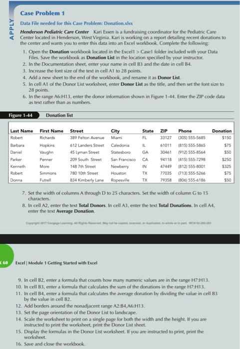
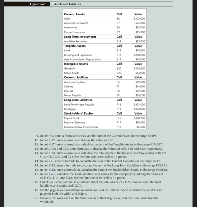
APPLY Case Problem 1 Data File needed for this Case Problem: Donation.xlsx Henderson Pediatric Care Center Kari Essen is a fundraising coordinator for the Pediatric Care Center located in Henderson, West Virginia. Kari is working on a report detailing recent donations to the center and wants you to enter this data into an Excel workbook. Complete the following: 1. Open the Donation workbook located in the Excell > Casel folder included with your Data Files. Save the workbook as Donation List in the location specified by your instructor 2. In the Documentation sheet, enter your name in cell B3 and the date in cell B4. 3. Increase the font size of the text in cell A1 to 28 points. 4. Add a new sheet to the end of the workbook, and rename it as Donor List. 5. In cell A1 of the Donor List worksheet, enter Donor List as the title, and then set the font size to 28 points 6. In the range A6:H13, enter the donor information shown in Figure 1-44. Enter the ZIP code data as text rather than as numbers. Figure 1-44 Donation list Last Name Robert Barbara Daniel Parker Kenneth Robert Donna First Name Richards Hopkins Vaughn Penner More Simmons Futrell Street City 389 Felton Avenue Miami 612 Landers Street Caledonia 45 Lyman Street Statesboro 209 South Street San Francisco 1487th Street Newberry 780 10th Street Houston 834 Kimberly Lane Ropesville State FL IL GA CA IN TX TX ZIP 33127 61011 30461 94118 47449 77035 79358 Phone (305) 555-5685 (815) 555-5865 1912) 555-8564 (415) 555-7298 (812) 555-8001 (713) 555-5266 (806) 555-6186 Donation $150 $75 $50 $250 $325 $75 $50 7. Set the width of columns A through D to 25 characters. Set the width of column G to 15 characters. 8. In cell A2, enter the text Total Donors. In cell A3, enter the text Total Donations. In cell A4, enter the text Average Donation Copyright 2017 Cangage Learning. All Rights Reserved. May not be copied, scanned, or duplicated, in whole or in part WCN 12-200-200 60 Excel Module 1 Getting Started with Excel 9. In cell B2, enter a formula that counts how many numeric values are in the range H7:H13. 10. In cell B3, enter a formula that calculates the sum of the donations in the range H7:H13. 11. In cell B4, enter a formula that calculates the average donation by dividing the value in cell B3 by the value in cell B2. 12. Add borders around the nonadjacent range A2:B4,46:H13. 13. Set the page orientation of the Donor List to landscape. 14. Scale the worksheet to print on a single page for both the width and the height. If you are instructed to print the worksheet, print the Donor List sheet. 15. Display the formulas in the Donor List worksheet. If you are instructed to print, print the worksheet 16. Save and close the workbook. CREATE Case Problem 2 Data File needed for this Case Problem: Balance.xlsx Scott Kahne Tool & Die Cheryl Hippe is a financial officer at Scott Kahne Tool & Die, a manufacturing company located in Mankato, Minnesota. Every month the company publishes a balance sheet, a report that details the company's assets and liabilities. Cheryl asked you to create the workbook with the text and formulas for this report. Complete the following: 1. Open the Balance workbook located in the Excel1 > Case2 folder included with your Data Files. Save the workbook as Balance Sheet in the location specified by your instructor 2. In the Documentation sheet, enter your name in cell B3 and the date in cell B4. 3. Go to the Balance Sheet worksheet. Set the font size of the title in cell A1 to 28 points. 4. In cell A2, enter the text Statement for March 2017 5. Set the width of columns A and Eto 30 characters. Set the width of columns B, C, E, and to 12 characters. Set the width of column D to 4 characters. (Hint: Hold down the Ctrl key as you click the column headings to select both adjacent and nonadjacent columns.) 6. Set the font size of the text in cells A4, C4, E4, and G4 to 18 points. 7. Set the font size of the text in cells A5, E5, A11, E11, A14, E15, A19, 20, and A24 to 14 points. 8. Enter the values shown in Figure 1-45 in the specified cells. Figure 1-45 Assets and liabilities Cell B6 B7 BB B9 Cell B12 Cell B15 B16 317 Current Assets Cash Accounts Receivable Inventories Prepaid Insurance Long-Term Investments Available Securities Tangible Assets Land Building and Equipment Less Accumulated Depreciation Intangible Assets Goodwill Other Assets Current Liabilities Accounts Payable Salaries Interest Notes Payable Long-Term Liabilities Long-Term Notes Payable Mortgage Stockholders' Equity Capital Stock Retained Earnings Comprehensive Income/Loss Cell 320 B22 Cell F6 F7 FB F9 Cell F12 F13 Cell F16 F17 F18 Value $123,000 $75,000 $58,000 $15,000 Value $29.000 Value $49,000 $188,000 -$48.000 Value $148,000 $14,000 Value $62,000 $14,000 $12.000 $38,000 Value $151,000 $103,000 Value $178,000 $98,000 -$5,000 9. In cell C9, enter a formula to calculate the sum of the Current Assets in the range B6:39. 10. In cell C12, enter a formula to display the value of B12. 11. In cell C17, enter a formula to calculate the sum of the Tangible Assets in the range B15:317. 12. In cells C20 and C22, enter formulas to display the values of cells B20 and B22, respectively. 13. In cell C24, enter a formula to calculate the total assets in the balance sheet by adding cells C9, C12, C17, C20, and C22. Set the font size of the cell to 14 points. 14. In cell G9, enter a formula to calculate the sum of the Current Liabilities in the range F6:F9. 15. In cell G13, enter a formula to calculate the sum of the Long-Term Liabilities in the range F12:F13. 16. In cell G18, enter a formula to calculate the sum of the Stockholders' Equity in the range F16:F18. 17. In cell G20, calculate the Total Liabilities and Equity for the company by adding the values of cells G9, G13, and G18. Set the font size of the cell to 14 points. 18. Check your calculations. In a balance sheet the total assets (cell C24) should equal the total liabilities and equity (cell G20). 19. Set the page layout orientation to landscape and the Balance Sheet worksheet to print to one page for both the width and height. 20. Preview the worksheet on the Print screen in Backstage view, and then save and close the workbook


