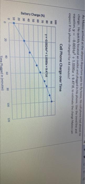
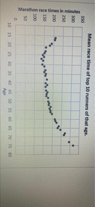
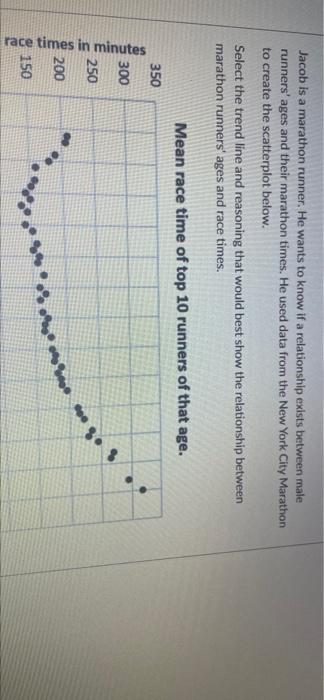
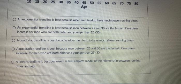
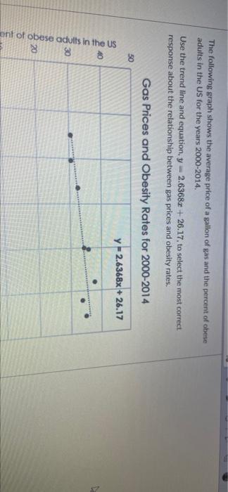
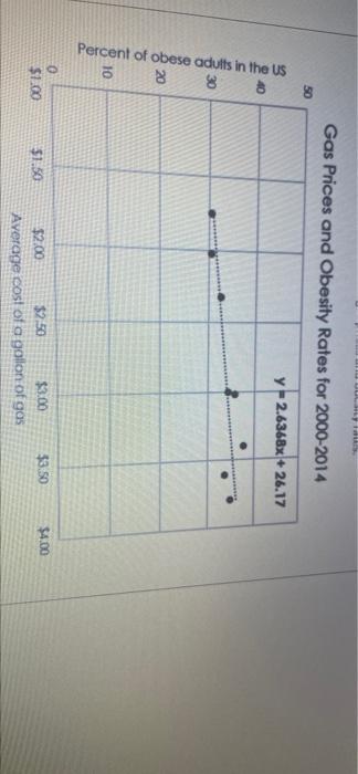
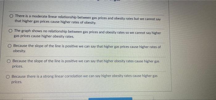
As Mateo arrived at the airport departure gate to fly home, his cell phone had almost no charge. He quickly located an outlet and plugged in his phone. Use the trend line and equation, y = -0.00242 +1.05952 + 9.4716, to estimate the charge Mateo can expect If his phone charged for 44 minutes? Cell Phone Charge over Time 100 90 80 70 60 50 y-0.0024x+1.0595% +9.4716 Battery Charge (36) 40 Ree 30 20 10 100 120 0 20 40 60 80 Time Plugged In (minutes) BI 20 10 0 20 100 120 40 60 80 Time Plugged In (minutes) (Round your answer to one decimal place, and don't include the % symbol.) Mean race time of top 10 runners of that age. 350 300 250 200 o 9 Marathon race times in minutes . 9 150 sono 5 100 50 o 10 15 20 25 30 35 40 45 50 55 60 65 70 75 80 Age Jacob is a marathon runner. He wants to know if a relationship exists between male runners' ages and their marathon times. He used data from the New York City Marathon to create the scatterplot below. Select the trend line and reasoning that would best show the relationship between marathon runners' ages and race times. Mean race time of top 10 runners of that age. 350 300 250 race times in minutes 200 2 o g. . 150 10 15 20 25 30 35 40 45 Age 50 55 60 65 70 75 80 An exponential trendline is best because older men tend to have much slower running times. An exponential trendline is best because men between 25 and 30 are the fastest. Race times increase for men who are both older and younger than 25-30. O A quadratic trendline is best because older men tend to have much slower running times. A quadratic trendline is best because men between 25 and 30 are the fastest. Race times increase for men who are both older and younger than 25-30. A linear trendline is best because it is the simplest model of the relationship between running times and age The following graph shows the average price of a gallon of gas and the percent of obese adults in the US for the years 2000-2014 Use the trend line and equation, y = 2.6368x + 26.17, to select the most correct response about the relationship between gas prices and obesity rates. Gas Prices and Obesity Rates for 2000-2014 50 y -2.6368x + 26.17 40 30 ont of obese adults in the US 20 Gas Prices and Obesity Rates for 2000-2014 50 y-2.6368x + 26.17 40 30 Percent of obese adults in the US 20 10 0 $1.00 $1.50 $3.50 $4.00 $2.00 $2.50 $3.00 Average cost of a gollon of gas There is a moderate linear relationship between gas prices and obesity rates but we cannot say that higher gas prices cause higher rates of obesity. The graph shows no relationship between gas prices and obesity rates so we cannot say higher gas prices cause higher obesity rates. Because the slope of the line is positive we can say that higher gas prices cause higher rates of obesity. Because the slope of the line is positive we can say that higher obesity rates cause higher gas prices Because there is a strong linear correlation we can say higher obesity rates cause higher gas prices
