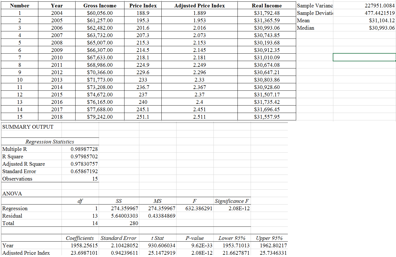
Assume that Mrs. Cooks real income will not change over the next ten years. Use the mean real income from previous steps to determine projected real income for the future ten years of Mrs. Cooks work expectancy. Use the regression equation from hint 2 to project adjusted price indices for the next ten years. Assume that Mrs. Cook pays 20% of her actual income in taxes and that Green will not provide significant state assistance. Use the projected real income and adjusted price indices to estimate Mrs. Cooks net actual income for the next ten years (2019-2028). What would be the likely amount of an award to Mrs. Cook based on a present value rate of 8%? Discuss the factors that could cause Mrs. Cooks future income to differ from your estimate.

Number 1 2 3 Year 2004 2005 Sample Varianc Sample Deviati Mean Median 227951.0084 477.4421519 $31,104.12 $30,993.06 2006 4 2007 2008 5 2009 6 7 Gross Income $60,056.00 $61,257.00 $62,482.00 $63,732.00 $65,007.00 $66,307.00 $67,633.00 $68,986.00 $70,366.00 $71,773.00 $73,208.00 $74,672.00 $76,165.00 $77,688.00 $79,242.00 Price Index 188.9 195.3 201.6 207.3 215.3 214.5 218.1 224.9 229.6 233 236.7 237 240 245.1 251.1 Adjusted Price Index 1.889 1.953 2.016 2.073 2.153 2.145 2.181 2.249 2.296 2.33 2.367 2.37 2.4 2.451 2.511 2010 2011 2012 2013 2014 2015 2016 2017 2018 Real Income $31,792.48 $31,365.59 $30,993.06 $30,743.85 $30,193.68 $30,912.35 $31,010.09 $30,674.08 $30,647.21 $30,803.86 $30,928.60 $31,507.17 $31,735.42 $31,696.45 $31,557.95 8 9 10 11 12 13 14 15 SUMMARY OUTPUT Regression Statistics Multiple R 0.98987728 R Square 0.97985702 Adjusted R Square 0.97830757 Standard Error 0.65867192 Observations 15 ANOVA df F Significance F 632.386291 2.08E-12 1 Regression Residual Total SS 274.359967 5.64003303 280 MS 274.359967 0.43384869 13 14 Year Adjusted Price Index Coefficients Standard Error 1958.25615 2.10428052 23.6987101 0.94239611 t Stat 930.606034 25.1472919 P-value 9.62E-33 2.08E-12 Lower 95% 1953.71013 21.6627871 Upper 95% 1962.80217 25.7346331 Number 1 2 3 Year 2004 2005 Sample Varianc Sample Deviati Mean Median 227951.0084 477.4421519 $31,104.12 $30,993.06 2006 4 2007 2008 5 2009 6 7 Gross Income $60,056.00 $61,257.00 $62,482.00 $63,732.00 $65,007.00 $66,307.00 $67,633.00 $68,986.00 $70,366.00 $71,773.00 $73,208.00 $74,672.00 $76,165.00 $77,688.00 $79,242.00 Price Index 188.9 195.3 201.6 207.3 215.3 214.5 218.1 224.9 229.6 233 236.7 237 240 245.1 251.1 Adjusted Price Index 1.889 1.953 2.016 2.073 2.153 2.145 2.181 2.249 2.296 2.33 2.367 2.37 2.4 2.451 2.511 2010 2011 2012 2013 2014 2015 2016 2017 2018 Real Income $31,792.48 $31,365.59 $30,993.06 $30,743.85 $30,193.68 $30,912.35 $31,010.09 $30,674.08 $30,647.21 $30,803.86 $30,928.60 $31,507.17 $31,735.42 $31,696.45 $31,557.95 8 9 10 11 12 13 14 15 SUMMARY OUTPUT Regression Statistics Multiple R 0.98987728 R Square 0.97985702 Adjusted R Square 0.97830757 Standard Error 0.65867192 Observations 15 ANOVA df F Significance F 632.386291 2.08E-12 1 Regression Residual Total SS 274.359967 5.64003303 280 MS 274.359967 0.43384869 13 14 Year Adjusted Price Index Coefficients Standard Error 1958.25615 2.10428052 23.6987101 0.94239611 t Stat 930.606034 25.1472919 P-value 9.62E-33 2.08E-12 Lower 95% 1953.71013 21.6627871 Upper 95% 1962.80217 25.7346331


