

Answered step by step
Verified Expert Solution
Question
1 Approved Answer
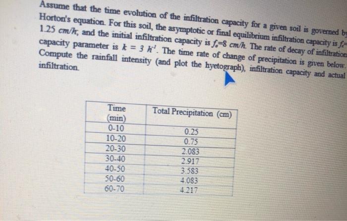
Assume that the time evolution of the infiltration capacity for a given soil is governed by Horton's equation. For this soil, the asymptotic or final
Step by Step Solution
There are 3 Steps involved in it
Step: 1

Get Instant Access to Expert-Tailored Solutions
See step-by-step solutions with expert insights and AI powered tools for academic success
Step: 2

Step: 3
Ace Your Homework with AI
Get the answers you need in no time with our AI-driven, step-by-step assistance
Get Started
Social Media Audit Measure For Impact
Authors: Urs E. Gattiker
2013 Edition
1461436028, 978-1461436027