at the one at d) the flash covers "E1"

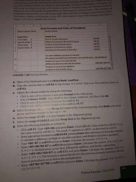
realize that you should avoid values in formulas most of the time. Therefore, you create that contains values you will use in your formulas. To test your knowledge of formulas will create an output area that will contain a variety of formules using cell references from the input area. You will include a formatted uitle the date neared, and your name. After creating and verifying formula results, you will change input values and observe changes in the formule results. You want to display cell formulas, so you will create a picture copy of the formulas view. Reler to Figure 1.60 as you complete this exercise. Excel Formulas and Order of Precedence Student Name 2 Date Created: 42614 4 Input Area: 5 First Value 2 6 Second Value 4 7 Third Value 6 8 Fourth Value S Output Area: Sum of 1st and 2nd values Difference between 4th and ist values Product of 2nd and and values Quotient of 3rd and 1st values 2nd value to the power of and value 1687 87/15 0687 1st value added to product of 2nd and 4th values and difference between sum and Brd value -85*38-87 Product of sum of 1st and 2nd and difference between 4th and Brd values (516) B-B Product of 1st and 2nd added to product of 3rd and 4th values BS 8687888 Excel 2014. Window FIGURE 1.60 Formula Practice a. Open Ipl Math and save it as e0lp1 Math Last First. b. Type the current date in cell B2 in this format: 9/1/2018. Type your first and last names in cell D2. c. Adjust the column widths by doing the following: Click in any cell in column A and click Format in the Cells group. . Select Column Width. Ive 12.57 in the Column width box, and then click OK Click in any cell in column B and set the width to 11. Click in any cell in columna D and set the width to 35.57. d. Select the range Al e k Merge & Center in the Alignment group, click Bold in the For group, and then change the font size to 14. e. Select the range B5:38 and click Center in the Alignment group. f. Select the range D10:D12 and click Wrap Text in the Alignment group. 8. Enter the following formulas in column E! Click cell E5. Type=B5+B6 and press Enter. Excel adds the value stored in cell B5 (1) to the value stored in cell B6 (2). The result (3) appears in cell E5, as described in cell 05 Enter appropriate formulas in cells E6:E8 pressing Enter after entering each formula Subtract to calculate a difference, multiply to calculate a product, and divide to calculate a quotient Type=B6 B7 in cell E9 and press Enter. Calculate the answer: 222 = 8. Enter =B5+B6 B8-B7 in cell E10 and press Enter. Calculate the answer: 2*4 = 8:1+8 9:9-3 = 6. Multiplication occurs first, followed by addition, and finally subtraction Enter =(B5+B6)*(B8-B7) in cell E11 and press Enter. Calculate the answer: 1+2 = 3: 4-3 = 1:31 = 3. This formula is almost identical to the previous formula: however, calcula- tions in parentheses occur before the multiplication. Enter =B5 B6+B7B8 in cell E12 and press Enter. Calculate the answer: 1'2 = 2: 394 = 12:2+12 = 14. 139 Practice Exercises. Excel 2016 h. Edit a formula and the input values: . Click cell El 2 and click in the Formula Bar to edit the formula. Add parentheses as shown: (B5 B6)+(B7'B8) and click Enter to the left side of the Formula Bar. The answer is still 14. The parentheses do not affect order of operations because multiplication occurred before the addition. The parentheses help improve the readability of the formula Type 2 in cell B5.4 in cell B6, 6 in cell B7 and 8 in cell B8. Double-check the results of the formulas using a calculator or your head. The new results in cells E5:E12 should be 6. 6. 24. 3. 4096, 28. 12. and 56, respectively 1. Double-click the Sheetl tab, type Results, and then press Enter. Right click the Results sheet tab, select Move or Copy, click (move to end) in the Before sheet section, click the Create a copy check box to select it, and click OK. Double-click the Results (2) sheet tab. type Formulas, and then press Enter. 1. Ensure that the Formulas sheet tab is active, click the Formulas sheet tab and click Show Formulas in the Formula Auditing group. Double-click between the column A and column B headings to adjust the column A width. Double-click between the column B and column headings to adjust the column B width. Set 24.00 width for column D. k. Ensure that the Formulas worksheet is active, click the Page Layout tab, and do the following: . Click the Gridlines Print check box to select it in the Sheet Options group. Click the Headings Print check box to select it in the Sheet Options group. 1. Click the Results sheet tab, press and hold Ctrl, and click the Formulas sheet tab to select both worksheets. Do the following: Click Orientation in the Page Setup group and select Landscape, . Click the Insert tab, click Header & Footer in the Text group. Click Go to Footer in the Navigation group. Type your name on the left side of the footer. Click in the center section of the footer and click Sheet Name in the Header & Footer Elements group. Click in the right section of the footer and click File Name in the Header & Footer elements group. m. Click in the worksheet, press Ctrl+Home, and click Normal View on the status bar. n. Click the File tab and click Print. Verify that each worksheet will print on one page. Press Ese to close the Print Preview, and right-click the worksheet tab and click Ungroup Sheets. o. Save and close the file. Based on your instructor's directions, submit colpi Math_LastFirst. tinn realize that you should avoid values in formulas most of the time. Therefore, you create that contains values you will use in your formulas. To test your knowledge of formulas will create an output area that will contain a variety of formules using cell references from the input area. You will include a formatted uitle the date neared, and your name. After creating and verifying formula results, you will change input values and observe changes in the formule results. You want to display cell formulas, so you will create a picture copy of the formulas view. Reler to Figure 1.60 as you complete this exercise. Excel Formulas and Order of Precedence Student Name 2 Date Created: 42614 4 Input Area: 5 First Value 2 6 Second Value 4 7 Third Value 6 8 Fourth Value S Output Area: Sum of 1st and 2nd values Difference between 4th and ist values Product of 2nd and and values Quotient of 3rd and 1st values 2nd value to the power of and value 1687 87/15 0687 1st value added to product of 2nd and 4th values and difference between sum and Brd value -85*38-87 Product of sum of 1st and 2nd and difference between 4th and Brd values (516) B-B Product of 1st and 2nd added to product of 3rd and 4th values BS 8687888 Excel 2014. Window FIGURE 1.60 Formula Practice a. Open Ipl Math and save it as e0lp1 Math Last First. b. Type the current date in cell B2 in this format: 9/1/2018. Type your first and last names in cell D2. c. Adjust the column widths by doing the following: Click in any cell in column A and click Format in the Cells group. . Select Column Width. Ive 12.57 in the Column width box, and then click OK Click in any cell in column B and set the width to 11. Click in any cell in columna D and set the width to 35.57. d. Select the range Al e k Merge & Center in the Alignment group, click Bold in the For group, and then change the font size to 14. e. Select the range B5:38 and click Center in the Alignment group. f. Select the range D10:D12 and click Wrap Text in the Alignment group. 8. Enter the following formulas in column E! Click cell E5. Type=B5+B6 and press Enter. Excel adds the value stored in cell B5 (1) to the value stored in cell B6 (2). The result (3) appears in cell E5, as described in cell 05 Enter appropriate formulas in cells E6:E8 pressing Enter after entering each formula Subtract to calculate a difference, multiply to calculate a product, and divide to calculate a quotient Type=B6 B7 in cell E9 and press Enter. Calculate the answer: 222 = 8. Enter =B5+B6 B8-B7 in cell E10 and press Enter. Calculate the answer: 2*4 = 8:1+8 9:9-3 = 6. Multiplication occurs first, followed by addition, and finally subtraction Enter =(B5+B6)*(B8-B7) in cell E11 and press Enter. Calculate the answer: 1+2 = 3: 4-3 = 1:31 = 3. This formula is almost identical to the previous formula: however, calcula- tions in parentheses occur before the multiplication. Enter =B5 B6+B7B8 in cell E12 and press Enter. Calculate the answer: 1'2 = 2: 394 = 12:2+12 = 14. 139 Practice Exercises. Excel 2016 h. Edit a formula and the input values: . Click cell El 2 and click in the Formula Bar to edit the formula. Add parentheses as shown: (B5 B6)+(B7'B8) and click Enter to the left side of the Formula Bar. The answer is still 14. The parentheses do not affect order of operations because multiplication occurred before the addition. The parentheses help improve the readability of the formula Type 2 in cell B5.4 in cell B6, 6 in cell B7 and 8 in cell B8. Double-check the results of the formulas using a calculator or your head. The new results in cells E5:E12 should be 6. 6. 24. 3. 4096, 28. 12. and 56, respectively 1. Double-click the Sheetl tab, type Results, and then press Enter. Right click the Results sheet tab, select Move or Copy, click (move to end) in the Before sheet section, click the Create a copy check box to select it, and click OK. Double-click the Results (2) sheet tab. type Formulas, and then press Enter. 1. Ensure that the Formulas sheet tab is active, click the Formulas sheet tab and click Show Formulas in the Formula Auditing group. Double-click between the column A and column B headings to adjust the column A width. Double-click between the column B and column headings to adjust the column B width. Set 24.00 width for column D. k. Ensure that the Formulas worksheet is active, click the Page Layout tab, and do the following: . Click the Gridlines Print check box to select it in the Sheet Options group. Click the Headings Print check box to select it in the Sheet Options group. 1. Click the Results sheet tab, press and hold Ctrl, and click the Formulas sheet tab to select both worksheets. Do the following: Click Orientation in the Page Setup group and select Landscape, . Click the Insert tab, click Header & Footer in the Text group. Click Go to Footer in the Navigation group. Type your name on the left side of the footer. Click in the center section of the footer and click Sheet Name in the Header & Footer Elements group. Click in the right section of the footer and click File Name in the Header & Footer elements group. m. Click in the worksheet, press Ctrl+Home, and click Normal View on the status bar. n. Click the File tab and click Print. Verify that each worksheet will print on one page. Press Ese to close the Print Preview, and right-click the worksheet tab and click Ungroup Sheets. o. Save and close the file. Based on your instructor's directions, submit colpi Math_LastFirst. tinn