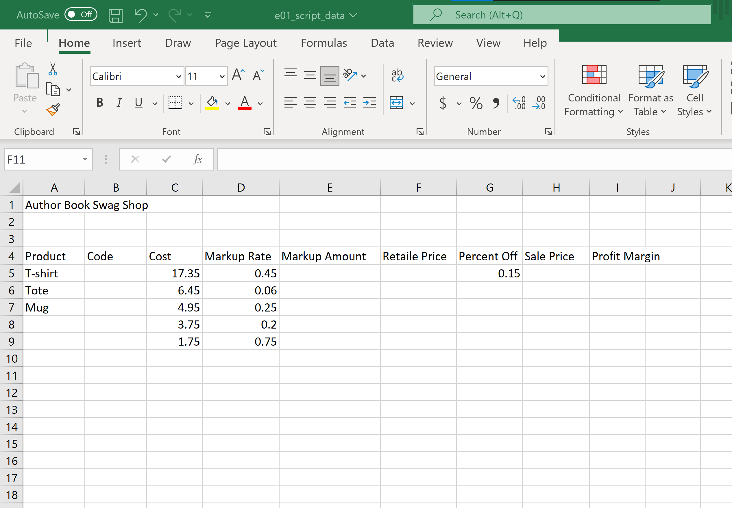
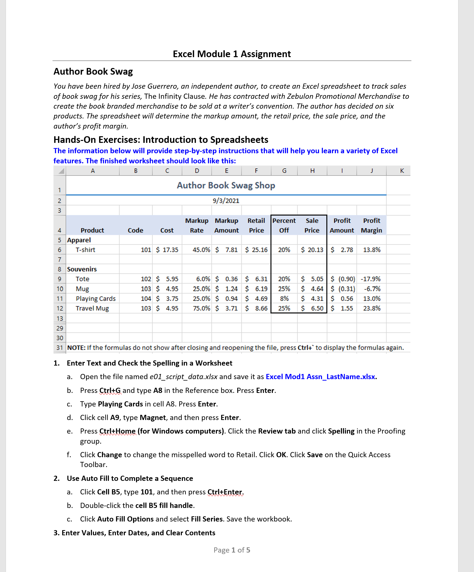
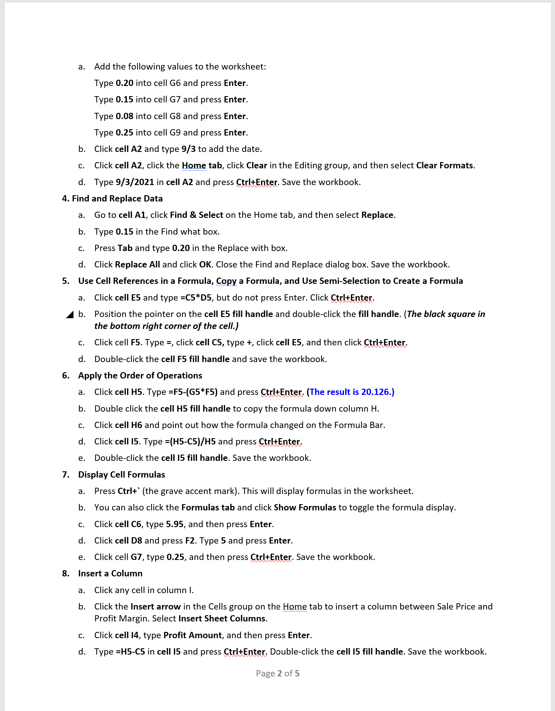
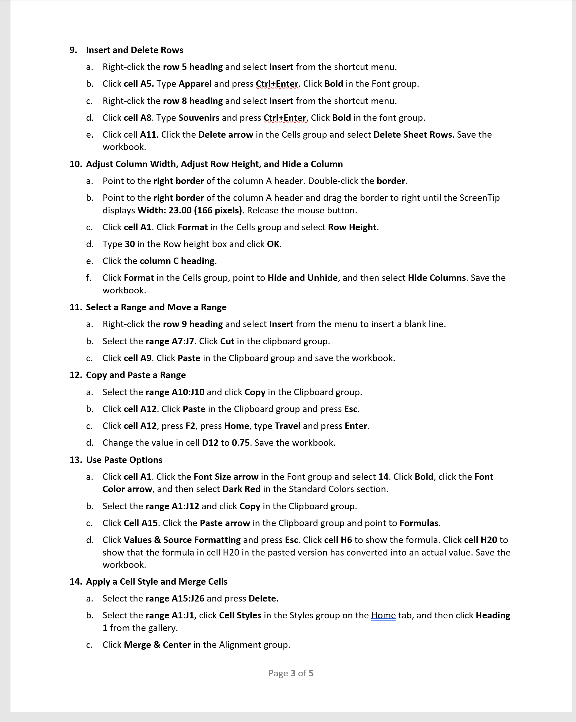
AutoSave (O Off) e01_script_data v Search (Alt +Q) File Home Insert Draw Page Layout Formulas Data Review View Help Calibri v 11 AA ap General Paste BIUV V v E v $ ~ % " .00 Conditional Format as Cell Formatting v Table Styles v Clipboard Font Alignment Number Styles F11 X V fx A B C D E F G H 1 Author Book Swag Shop IN W 4 Product Code Cost Markup Rate Markup Amount Retaile Price Percent Off Sale Price Profit Margin 5 T-shirt 17.35 0.45 0.15 6 Tote 6.45 0.06 7 Mug 4.95 0.25 8 3.75 0.2 9 1.75 0.75 10 11 12 13 14 15 16 17 18Excel Module 1 Assignment Author Book Swag You have been hired by Jose Guerrero, an independent author, to create an Excel spreadsheet to track sales of book swag for his series, The Infinity Clause. He has contracted with Zebulon Promotional Merchandise to create the book branded merchandise to be sold at a writer's convention. The author has decided on six products. The spreadsheet will determine the markup amount, the retail price, the sale price, and the author's profit margin. Hands-On Exercises: Introduction to Spreadsheets The information below will provide step-by-step instructions that will help you learn a variety of Excel features. The finished worksheet should look like this: A B C D E F G H J K Author Book Swag Shop 2 9/3/2021 3 Markup Markup Retail Profit Profit 4 Product Code Cost Rate Amount Price Amount Margin 5 Apparel 6 T-shirt 101 $17.35 45.0% S 7.81 5 25.16 S 2.78 13.8% 7 8 Souvenirs 9 Tote 102 S 5.95 6.0% S 0.36 S 6.31 S (0.90) 47.9% 10 Mug 103 s 4.95 25.0% s 1.24 s 6.19 s (0.31) -6.7% 11 PIayingCards 104$ 3.75 25.0% S 0.94 S 4.69 S 0.56 13.0% 12 TravelMug 103 S 4.95 75.0% S 3.71 S 8.66 S 1.55 23.8% 13 29 30 31 NOTE: If the formulas do not show after closing and reopening the file, press Ctr|+' to display the formulas again. 1. Enter Text and Check the Spelling in a Worksheet a. Open the file named e01_script_data.xlsx and save it as Excel Modl Assn_LastName.xst. b. Press Wand type A8 in the Reference box. Press Enter. c. Type Playing Cards in cell A8. Press Enter. d. Click cell A9, type Magnet, and then press Enter. e. Press W (for Windows computers). Click the Review tab and click Spelling in the Proofing group. f. Click Change to change the misspelled word to Retail. Click OK. Click Save on the Quick Access Toolbar. 2. Use Auto Fill to Complete a Sequence a. Click Cell BS, type 101, and then press 513% b. Doubleclick the cell B5 fill handle. c. Click Auto Fill Options and select Fill Series. Save the workbook. 3. Enter Values, Enter Dates, and Clear Contents Page 1 of 5 b. c. d. Add the following values to the worksheet: Type 0.20 into cell 66 and press Enter. Type 0.15 into cell G7 and press Enter. Type 0.08 into cell 68 and press Enter. Type 0.25 into cell 69 and press Enter. Click cell A2 and type 9/3 to add the date. Click cell A2, click the Hog tab, click Clear in the Editing group, and then select Clear Formats. Type 9/3/2021 in cell A2 and press W. Save the workbook. 4. Find and Replace Data a. b. c. d. Go to cell A1, click Find & Select on the Home tab, and then select Replace. Type 0.15 in the Find what box. Press Tab and type 0.20 in the Replace with box. Click Replace All and click OK. Close the Find and Replace dialog box. Save the workbook. 5. Use Cell References in a Formula, City a Formula, and Use Semi-Selection to Create a Formula a. Ab. C. d. Click cell E5 and type =C5*D5, but do not press Enter. Click W. Position the pointer on the cell E5 fill handle and doubleclick the fill handle. (The black square in the bottom right corner of the cell.) Click cell F5. Type =, click cell C5, type +, click cell E5, and then clickm Doubleclick the cell F5 fill handle and save the workbook. 6. Apply the Order of Operations a. b. c. cl. e. Click cell H5. Type =F5-(G5*F5) and press mm (The result is 20.126.) Double click the cell H5 fill handle to copy the formula down column H. Click cell H6 and point out how the formula changed on the Formula Bar. Click cell l5. Type =(H5-C5)/H5 and press m Doubleclick the cell I5 fill handle. Save the workbook. 7. Display Cell Formulas a. b. c. d. e. Press Ctrl+' (the grave accent mark). This will display formulas in the worksheet. You can also click the Formulas tab and click Show Formulas to toggle the formula display. Click cell C6, type 5.95, and then press Enter. Click cell D8 and press F2. Type 5 and press Enter. Click cell G7, type 0.25, and then press W- Save the workbook. 8. Insert a Column a. b. Click any cell in column |. Click the Insert arrow in the Cells group on the Hometab to insert a column between Sale Price and Profit Margin. Select Insert Sheet Columns. Click cell l4, type Profit Amount, and then press Enter. Type =H5-C5 in cell I5 and press m Doubleclick the cell I5 fill handle. Save the workbook. Page 2 of 5 Insert and Delete Rows Right-click the row 5 heading and select Insert from the shortcut menu. Click cell A5. Type Apparel and press W. Click Bold in the Font group. Rightclick the row 8 heading and select Insert from the shortcut menu. Click cell A8. Type Souvenirs and press m Click Bold in the font group. Click cell All. Click the Delete arrow in the Cells group and select Delete Sheet Rows. Save the workbook. 10. Adjust Column Width, Adjust Row Height, and Hide a Column 0- o 5\" Point to the right border of the column A header. Doubleclick the border. Point to the right border of the column A header and drag the border to right until the ScreenTip displays Width: 23.00 (166 pixels). Release the mouse button. Click cell A1. Click Format in the Cells group and select Row Height. Type 30 in the Row height box and click OK. Click the column C heading. Click Format in the Cells group, point to Hide and Unhide, and then select Hide Columns. Save the workbook. 11. Select a Range and Move a Range a. b. C. Rightclick the row 9 heading and select Insert from the menu to insert a blank line. Select the range A7:J7. Click Cut in the clipboard group. Click cell A9. Click Paste in the Clipboard group and save the workbook. 12. Copy and Paste a Range a. b. c. d. Select the range A10:J10 and click Copy in the Clipboard group. Click cell A12. Click Paste in the Clipboard group and press Esc. Click ce|| A12, press F2, press Home, type Travel and press Enter. Change the value in cell D12 to 0.75. Save the workbook. 13. Use Paste Options a. Click cell A1. Click the Font Size arrow in the Font group and select 14. Click Bold, click the Font Color arrow, and then select Dark Red in the Standard Colors section. Select the range A1:112 and click Copy in the Clipboard group. Click Cell A15. Click the Paste arrow in the Clipboard group and point to Formulas. Click Values & Source Formatting and press Esc. Click cell H6 to show the formula. Click cell H20 to show that the formula in cell H20 in the pasted version has converted into an actual value. Save the workbook. 14. Apply a Cell Style and Merge Cells Select the range A15:J26 and press Delete. Select the range A1:11, click Cell Styles in the Styles group on the Hometab, and then click Heading 1 from the gallery. Click Merge & Center in the Alignment group. Page 3 of 5 15. 16. 17. 18. 19. d. Select the range A2:JZ. Click Merge & Center. Save the workbook. Change Cell Alignment and Wrap Text a. b. C. Click cell A1 and click Middle Align in the Alignment group. Select the range A4:J4. Click Center in the Alignment group and click Bold in the Font group. Click Wrap Text in the Alignment group. Save the workbook. Increase Indent a. b. Select cell A6. Click Increase Indent in the Alignment group twice. Select the range A9:12 and click Increase Indent twice. Save the workbook. Apply a Border and Fill Color a. b. C. Select range A4:J4 and click the Fill Color arrow in the Font group. Click Blue, Accent 5, Lighter 80% (second row, column nine). Select the range G4:H12, click the Border arrow in the Font group, and then select Thick Outside Borders. Click cell A4. Save the workbook. Apply Number Formats and Increase and Decrease Decimal Places Select columns B:D. Click Format in the Cells group. Click Hide 8: Unhicle. Click Unhide Columns. Select ranges C62C12, E6:F12, and H6:|12. Click Accounting Number Format in the Number group. Select the ranges D6:DlZ and16:112. Click Percent Style in the Number group. Click Increase Decimal in the Number group. Select the range G6:G12, click Percent Style, and then click Center. Select the range 16:112, click Align Right, and then click Increase Indent. Save the workbook. Copy, Move, and Rename a Worksheet Rightclick the Sheetl tab. Select Move or Copy. Click the Create a copy check box and click OK. Drag the Sheetl (2) worksheet tab to the right of the Sheetl worksheet tab. Doubleclick the Sheetl sheet tab, type September, and then press Enter. Rename Sheetl (2) as Formulas. Press Ctrl+' to display formulas in the Formula worksheet. Change these column widths in the Formulas sheet: I Column A: 15.00 0 Column C, D, E, F, H, l, and J: 8.00 0 Column 6: 7.00 Click cell A31. Type NOTE: If the formulas do not show after closing and reopening the file, press Ctrl+' to display the formulas again. Select the range A31:K31. Click the Merge & Center arrow and click Merge Cells. Select the word Note and click Bold. Select Ctrl+' and click Bold. Save the workbook. Page 4 of 5 20. 21. 22. Set Page Orientation, Scaling, and Margin Options 3. Click the September sheet tab, press and hold Ctrl, and then click the Formulas sheet tab. b. Click the Page Layout tab, click Orientation in the Page Setup group, and then select Landscape. c. Click Margins. Select Custom Margins. d. Change the Top margin to 1". e. Click the Horizontally check box and click OK. f. Right-click the Formulas sheet tab and select Ungroup Sheets. With the Formulas sheet active, click the Page Setup Dialog Box Launcher in the Scale to Fit group. Click Fit to and click OK. Save the workbook. Create a Header a. Click the September sheet tab. Press and hold Ctrl and click the Formulas sheet tab. b. Click the Insert tab and click Header & Footer in the Text group. c. Click in the left section ofthe header and type Your Name. d. Click in the center section of the header and click Sheet Name. 9. Click in the right section ofthe header and click File Name. f. Click in any cell in the worksheet and click Normal in the status bar. g. Click cell A1, click the Review tab, and then click Spelling. Correct all errors and click OK when the spelling check completes. Leave the worksheets grouped. Save the workbook. View in Print Preview and Print a. Click the File tab and click Print. b. Verify the Printer box displays the printer you want to use to print the workbook. Verify the first Setting option displays Print Entire Workbook. Verify the last Settings option displays Fit Sheet on One Page. c. Click Next Page to see the second page. d. Click the Back arrow and save the workbook. e. Save and close the file. Exit Excel. Page 5 of 5