

Answered step by step
Verified Expert Solution
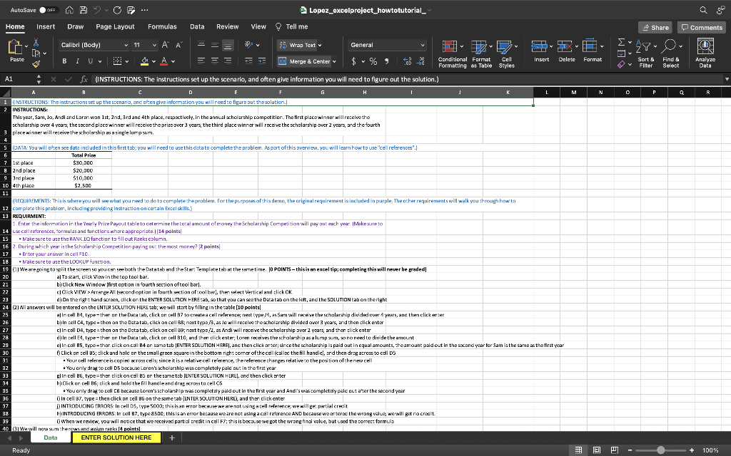
Question
1 Approved Answer
AutoSave OF AAOF... Lopez_excelproject_howtotutorial_ View Tell me Home Insert Draw Page Layout Formulas Data Review Share Comments Calibrl (Body) v 11 X G v A
AutoSave OF AAOF... Lopez_excelproject_howtotutorial_ View Tell me Home Insert Draw Page Layout Formulas Data Review Share Comments Calibrl (Body) v 11 X G v A A 25 Wrap Text General FO) v Paste YA Av - - = = = Insert Y Merge & Center v Delete Format Conditional Format Cell Formatting es Table Styles Sort Filter Find & Select Analyze Data D6 fx A P D G H I J L M N 0 P Q R S T U V Rank 1 2 3 4 First Year 5 Second Year Third Year 7 Fourth Year Scholarship Yearly Prize Payout Jo Andi $6,666.67 $10.000 56,667 $10,000 $6.657 Loren $2,500 $7,500 $7,500 $7,500 $7,500 Total $26,667 $ $24,167 $14,167 $ $7.500 2 3 1 9 10 During which year is the Schalarship Competition paying out the most money? 11 12 13 14 15 16 17 18 19 20 21 22 23 24 25 26 27 28 29 30 32 33 34 35 36 37 38 39 40 42 43 41 Data ENTER SOLUTION HERE + Ready + 100% Share Comments v FO) IN Analyze Data Insert Delete Format Y V Sort & Filter Find & Select AutoSave OF 2 OF Lopez_excelproject_howtotutorial_ Home Insert Draw Page Layout Formulas Data Review View Tell me X Calibrl (Body) v 11 ~ A ab Wrap Text General G Pastc BIU 17 YA = = $ - % Merge & Center % Conditional Format Cell Formatting es Table Styles A1 fx (INSTRUCTIONS: The instructions set up the scenario, and often give information you will need to figure out the solution.) A A R D E H I 1 ONSTRUCTIONS: The instructions set up the scenario, and often give information you will need to figure out the solution. 2 INSTRUCTIONS This year, Sam, lo, Andi and Laren wan 1st, 2nd, 3rd and 4th place, respectively, in the annual scholarship competition. The first place winner will receive the scholarship over 4 years, the second place winner will receive the prize over 3 years the third place winner will raceve the scholarship over 2 years, and the fourth 3 place winner will receive the scholarship as a single lumpsum. L M N 0 P Q R 5 (DATA: You will often see data included in this first tab; you will need to use this data to complete the problem. As part of this overview, you will learn how to use cell references". 6 Total Price 7 7 1st place $30,000 2nd place $20,000 9 3rd place $10,000 10 4th place $2,500 11 REQUIREMENTS: This is where you will see what you need to do tocomplete the problem. For the purposes of this demo, the original requirement is included in purple. The other requirements will walk you through how to 12 complete this problem, including providing instruction on certain Excel skills.) 13 REQUIRMENT: 1. Enter the information in the early Prize Payout tableta cetermine the total amount of money the Scholarship Competition will pay out each year Makesure to 14 Le cell references, formulas and functions where appropriate.(14 points 15 - Make sure to use the RANK.E function to fill out Ranks column. 16 2 Durire which year is the Scholarship Competition paying out the most money? 12 points 17 Enter your answer in cell F10 12 Wake sure to use the LOOKUP function. 19 We are going to split the screen so you can see both the Dalate and the Stars Templates at the same time. JO POINTS - this is an excel tip: completing this will never be graded 20 al Tastart, click View in the top toolbar. 21 b) Click New Window first option in fourth section oftcoltarl. 22 click VIEW > Arrange lisecond option in fourth section of toolbar), then select Vertical and click OK 23 di On the right hand screen, click on the ENTER SOLUTION HERE tab, so that you can see the Datatab on the left, and the SOLUTION tab ontheright 24 (2All answers will be entered on the ENTER SOLUTION HERE tab; we will start by fillinginthe table [10 points 25 alinel 4, type-ther on the Datatab, click on cell B7 to create cell reference next type 11. Sam will receive the scholarship divided over years, and then click entier 26 biln cell C4, type-then on the Datatab, click on cell 33; next types, as do will receive the scholarship divided over 3 years, and then click enter 27 ci in cell 04, type=then on the Datatab, click on cell 39; next type:2, as Andi will receive the scholarship over 2 years, and then click enter 28 d) In cell E4, type-ther on the Datab, click on tell 810, and then dickenler, Loren receives the scholarship as a lump sum, so no need to divide the amount 29 clinceles, type-then click on call 4 on sametab ENTER SOLUTION HERE), and then click anter; since the scholarship is paid out in equal amounts, the amount paid out in the second year for Sam is the same the first year 30 Click on cell 95; click and holc on the small green square in the bottom righ: comer ofthecell called the fill handic, and then drag arce to cell DS 31 - Your cell reference iscopie cross cells; since it is a relativecell reference, therelerence changes relative to the position of the new cell 32 . You only drag to call D5 because Loren's scholarship was completely paid out in the first year 33 In cell eG, type=then click on cells or the sametab ENTER SOLUTION HERE), and then click enter 34 h) Click or cell 16 dick and hold the fill handleand drag across to cell CS 35 . You only drag to cell C because Loren's scholarshi wax completely paid out in the first year and Andi's was completely paid out after the second year 36 i) in cell 37, type=then click on cell G on the same tab (ENTER SOLUTION HERE), and then click enter 37 1) INTRODUCING ERRORS- In cell 05, type 5000; this is an error because we are not using a cell reference; we will ge partial credit 38 h) INTRODUCING ERRORS. In cell B7, type 8500, this is an error because we are not using ace reference AND because we artered the wrong valuc, we will get acredit 39 1) When we review, you will notice that we received partial credit incel F7; this is because we got the wrong final value, but used the correct formula 40 Wawill now there and assipo anks points Data ENTER SOLUTION HERE + Ready + 100% Share Comments O , v FO) IN Analyze Data Insert Delete Format Y v Sort 9 Filter Find & Select K L M N 0 P Q R AutoSave OF 2 OF Lopez_excelproject_howtotutorial_ Home Insert Draw Page Layout Formulas Data Review View Tell me X Calibrl (Body) v 11 ~ A ab Wrap Text General G Pastc B I U 17 A Merge & Center $ % f Conditional Format Cell Formatting es Table Styles A1 fx (INSTRUCTIONS: The instructions set up the scenario, and often give information you will need to figure out the solution.) A R C D E F H 1 38 HINTRODUCING ERRORS: In cell 07, type 8500;this is an error because weare not using acel referente AND because we enters the wrong value, we will get no credit 39 1) When we review, you will notice that we received partial credit incl F7; this is because we got the wrang final value, but wed the correct formula 40 Vie will now therons and acign ranks (4 points 41 al in cell 4, type SUM34:14and then click Enter 42 b) Click or call F4;click and hold the till handle and drag dewr tacell F7 43 clincell G4, typc-RANK.EO4.$F$4:$F$7,01 44 The RANK.Eu function will assign the appropriate renk to the totals in column with 1 as the greatest total 45 Thesisused tacreate a salute calderice, or one that continuesta reference the exact same call no matter the relative position; we use this a we can drie 46 di click or call 54click and hold the till handic and drag down to cell 47 (4) Now, we will determine during which year the scholarship committee paid uut the most money (2 points] 48 All All Flotype-LOOKUP 1,6467,44:47) 49 The LOOKUP furction finds the call with a rank of 1 incis G4:G7, and then grabs thevaluc in the corresponding row incelis A4 A7 50 (SAVE & SUBMIT: After completing project, you need to save your salution spreadsheet, so that you can upload it to be auto-grade. Make sure you do not included acesin the file name, as this will keep the file from uploading 5. successfully 52 SAVE & SUBMIT: (1) After entering your answer in the secondtah (ENTER SOLLITION HERFI, Se your spredt by clicking FILE > SAVE AS. Make sure you DO NOT include: space in your file name, and 53 remember to save thetilcsorrowhere you will be able to find it, such as the Desktop 54 (2Return to the Project Window-where you initially downloader your spreadsheet to submit your solution for pradire. 55 d) You are now on stopdick Choose File 56 Select your updated spreadsheet, and click OK 57 Click Upload 58 El Click Submit for Grading 59 60 REVIEW RESULTS: 61 Ta see how you did, click on Results in My Accounting. Athen click on the signment, and the question you just submitted 62 FIRST ATTEMPTI AT THIS POINT YOU WILL SAVE YOUR FILE, RETURN TO THE PROJECT WINDOW, AND UPLOAD YOUR SUBMISSION FOR GRADING. REMEMBER TO RETURN TO THIS SPREADSHEET FOR YOUR SECOND ATTEMPT TO CORRECT ALL MISTAKES AND EARN 100%|| G3 64 65 GE SECOND ATTEMPTI CORRECT YOUR MISTAKES BY FOLLOWING THE STEPS BELOW, THEN RE-SUBMIT YOUR SOULTION TO RECEIVE 100%.11 67 fia 69 (Cpen the solution spreachect you saved for your first attempt 70 21 Correct tell DS in ENTER SOLUTION HERE tab; click on cell DS and type=24 71 (3) Correct cell R7 in ENTER SOLLION HERE tab. dick on cell 7 and type-R5 72 73 SAVE & SUBMIT: After entering your answer in the second tah (ENTER SOLLITION HERF), Save your spreadsheet by clicking FILE SAVE AS. Make sure you DO NOT include: spaces in your file name, and 74 remember to save the file somewhere you will be able to find it, such as the Desktop 75 (2) Return to the Project Window-where you initially downloader your spreadsheet -to submit your solution for grading. 76 All My Accountinglab, click on Assignments Do Homework Data ENTER SOLUTION HERE + Ready + 100% AutoSave OF 2 OF Lopez_excelproject_howtotutorial_ View Tell me Home Insert Draw Page Layout Formulas Data Review Share Comments Calibrl (Body) v 11 X G ~ A Wrap Text General , v FO) IN Analyze Data Paste Insert Delete Y Format v Sort & Filter Find & Select A1 BIU 17 A = = Merge & Center $ % ? Conditional Format Cell Formatting es Table Styles fx (INSTRUCTIONS: The instructions set up the scenario, and often give information you will need to figure out the solution.) D H A L M . N P Q R 62 FIRST ATTEMPT! AT THIS POINT YOU WILL SAVE YOUR FILE, RETURN TO THE PROJECT WINDOW, AND UPLOAD YOUR SUBMISSION FOR GRADING. REMEMBER TO RETURN TO THIS SPREADSHEET FOR YOUR SECOND ATTEMPT TO CORRECT ALL MISTAKES AND EARN 100%!! 63 64 GS 66 SECOND ATTEMPT! CORRECT YOUR MISTAKES BY FOLLOWING THE STEPS BELOW, THEN RE-SUBMIT YOUR SOULTION TO RECEIVE 100%!! 67 G2 (1 Open the solution prescsheet you saved for your first attempt 70 | Correct cells in ENTER SOLUTION HERE TAL; click on cells and type-04 72 Correct cell B7 in ENTER SOLUTION HERE tab, click on call e7 and type-BG 72 73 SAVE SUBMIT 01 Atter entering your answer in the second tab (ENTER SOLUTION HERE, save your spreadsheet by clicking FILE > SAVE AS. Make sure you DO NOT included paces in your file name, and 74 remember to save the file surrewhere you will be able to find it, such as the Desktup 75 Return to the Project Window-where yau initially downloaded your spreacher-ta submit your solution for gradire 76 alin My Accountinglab, click on Rezignments > Do Homework 27 bclickur the assignment 78 Click on the question you just submitted to apen a new attempt 75 di Skip to Step 3, and click Choose File 80 el Select your updated spreadsheet, and click Ok 81 Click pload 82 RlClick Submit for Grading 83 84 REVIEW RESULTS 85 To see how you did, click on Results in My AccountingLab;shen click on the assignment, and the question you just submitted. 86 87 82 09 90 91 92 93 94 95 96 97 98 99 100 101 102 Data ENTER SOLUTION HERE + Ready + 100% AutoSave OF AAOF... Lopez_excelproject_howtotutorial_ View Tell me Home Insert Draw Page Layout Formulas Data Review Share Comments Calibrl (Body) v 11 X G v A A 25 Wrap Text General FO) v Paste YA Av - - = = = Insert Y Merge & Center v Delete Format Conditional Format Cell Formatting es Table Styles Sort Filter Find & Select Analyze Data D6 fx A P D G H I J L M N 0 P Q R S T U V Rank 1 2 3 4 First Year 5 Second Year Third Year 7 Fourth Year Scholarship Yearly Prize Payout Jo Andi $6,666.67 $10.000 56,667 $10,000 $6.657 Loren $2,500 $7,500 $7,500 $7,500 $7,500 Total $26,667 $ $24,167 $14,167 $ $7.500 2 3 1 9 10 During which year is the Schalarship Competition paying out the most money? 11 12 13 14 15 16 17 18 19 20 21 22 23 24 25 26 27 28 29 30 32 33 34 35 36 37 38 39 40 42 43 41 Data ENTER SOLUTION HERE + Ready + 100% Share Comments v FO) IN Analyze Data Insert Delete Format Y V Sort & Filter Find & Select AutoSave OF 2 OF Lopez_excelproject_howtotutorial_ Home Insert Draw Page Layout Formulas Data Review View Tell me X Calibrl (Body) v 11 ~ A ab Wrap Text General G Pastc BIU 17 YA = = $ - % Merge & Center % Conditional Format Cell Formatting es Table Styles A1 fx (INSTRUCTIONS: The instructions set up the scenario, and often give information you will need to figure out the solution.) A A R D E H I 1 ONSTRUCTIONS: The instructions set up the scenario, and often give information you will need to figure out the solution. 2 INSTRUCTIONS This year, Sam, lo, Andi and Laren wan 1st, 2nd, 3rd and 4th place, respectively, in the annual scholarship competition. The first place winner will receive the scholarship over 4 years, the second place winner will receive the prize over 3 years the third place winner will raceve the scholarship over 2 years, and the fourth 3 place winner will receive the scholarship as a single lumpsum. L M N 0 P Q R 5 (DATA: You will often see data included in this first tab; you will need to use this data to complete the problem. As part of this overview, you will learn how to use cell references". 6 Total Price 7 7 1st place $30,000 2nd place $20,000 9 3rd place $10,000 10 4th place $2,500 11 REQUIREMENTS: This is where you will see what you need to do tocomplete the problem. For the purposes of this demo, the original requirement is included in purple. The other requirements will walk you through how to 12 complete this problem, including providing instruction on certain Excel skills.) 13 REQUIRMENT: 1. Enter the information in the early Prize Payout tableta cetermine the total amount of money the Scholarship Competition will pay out each year Makesure to 14 Le cell references, formulas and functions where appropriate.(14 points 15 - Make sure to use the RANK.E function to fill out Ranks column. 16 2 Durire which year is the Scholarship Competition paying out the most money? 12 points 17 Enter your answer in cell F10 12 Wake sure to use the LOOKUP function. 19 We are going to split the screen so you can see both the Dalate and the Stars Templates at the same time. JO POINTS - this is an excel tip: completing this will never be graded 20 al Tastart, click View in the top toolbar. 21 b) Click New Window first option in fourth section oftcoltarl. 22 click VIEW > Arrange lisecond option in fourth section of toolbar), then select Vertical and click OK 23 di On the right hand screen, click on the ENTER SOLUTION HERE tab, so that you can see the Datatab on the left, and the SOLUTION tab ontheright 24 (2All answers will be entered on the ENTER SOLUTION HERE tab; we will start by fillinginthe table [10 points 25 alinel 4, type-ther on the Datatab, click on cell B7 to create cell reference next type 11. Sam will receive the scholarship divided over years, and then click entier 26 biln cell C4, type-then on the Datatab, click on cell 33; next types, as do will receive the scholarship divided over 3 years, and then click enter 27 ci in cell 04, type=then on the Datatab, click on cell 39; next type:2, as Andi will receive the scholarship over 2 years, and then click enter 28 d) In cell E4, type-ther on the Datab, click on tell 810, and then dickenler, Loren receives the scholarship as a lump sum, so no need to divide the amount 29 clinceles, type-then click on call 4 on sametab ENTER SOLUTION HERE), and then click anter; since the scholarship is paid out in equal amounts, the amount paid out in the second year for Sam is the same the first year 30 Click on cell 95; click and holc on the small green square in the bottom righ: comer ofthecell called the fill handic, and then drag arce to cell DS 31 - Your cell reference iscopie cross cells; since it is a relativecell reference, therelerence changes relative to the position of the new cell 32 . You only drag to call D5 because Loren's scholarship was completely paid out in the first year 33 In cell eG, type=then click on cells or the sametab ENTER SOLUTION HERE), and then click enter 34 h) Click or cell 16 dick and hold the fill handleand drag across to cell CS 35 . You only drag to cell C because Loren's scholarshi wax completely paid out in the first year and Andi's was completely paid out after the second year 36 i) in cell 37, type=then click on cell G on the same tab (ENTER SOLUTION HERE), and then click enter 37 1) INTRODUCING ERRORS- In cell 05, type 5000; this is an error because we are not using a cell reference; we will ge partial credit 38 h) INTRODUCING ERRORS. In cell B7, type 8500, this is an error because we are not using ace reference AND because we artered the wrong valuc, we will get acredit 39 1) When we review, you will notice that we received partial credit incel F7; this is because we got the wrong final value, but used the correct formula 40 Wawill now there and assipo anks points Data ENTER SOLUTION HERE + Ready + 100% Share Comments O , v FO) IN Analyze Data Insert Delete Format Y v Sort 9 Filter Find & Select K L M N 0 P Q R AutoSave OF 2 OF Lopez_excelproject_howtotutorial_ Home Insert Draw Page Layout Formulas Data Review View Tell me X Calibrl (Body) v 11 ~ A ab Wrap Text General G Pastc B I U 17 A Merge & Center $ % f Conditional Format Cell Formatting es Table Styles A1 fx (INSTRUCTIONS: The instructions set up the scenario, and often give information you will need to figure out the solution.) A R C D E F H 1 38 HINTRODUCING ERRORS: In cell 07, type 8500;this is an error because weare not using acel referente AND because we enters the wrong value, we will get no credit 39 1) When we review, you will notice that we received partial credit incl F7; this is because we got the wrang final value, but wed the correct formula 40 Vie will now therons and acign ranks (4 points 41 al in cell 4, type SUM34:14and then click Enter 42 b) Click or call F4;click and hold the till handle and drag dewr tacell F7 43 clincell G4, typc-RANK.EO4.$F$4:$F$7,01 44 The RANK.Eu function will assign the appropriate renk to the totals in column with 1 as the greatest total 45 Thesisused tacreate a salute calderice, or one that continuesta reference the exact same call no matter the relative position; we use this a we can drie 46 di click or call 54click and hold the till handic and drag down to cell 47 (4) Now, we will determine during which year the scholarship committee paid uut the most money (2 points] 48 All All Flotype-LOOKUP 1,6467,44:47) 49 The LOOKUP furction finds the call with a rank of 1 incis G4:G7, and then grabs thevaluc in the corresponding row incelis A4 A7 50 (SAVE & SUBMIT: After completing project, you need to save your salution spreadsheet, so that you can upload it to be auto-grade. Make sure you do not included acesin the file name, as this will keep the file from uploading 5. successfully 52 SAVE & SUBMIT: (1) After entering your answer in the secondtah (ENTER SOLLITION HERFI, Se your spredt by clicking FILE > SAVE AS. Make sure you DO NOT include: space in your file name, and 53 remember to save thetilcsorrowhere you will be able to find it, such as the Desktop 54 (2Return to the Project Window-where you initially downloader your spreadsheet to submit your solution for pradire. 55 d) You are now on stopdick Choose File 56 Select your updated spreadsheet, and click OK 57 Click Upload 58 El Click Submit for Grading 59 60 REVIEW RESULTS: 61 Ta see how you did, click on Results in My Accounting. Athen click on the signment, and the question you just submitted 62 FIRST ATTEMPTI AT THIS POINT YOU WILL SAVE YOUR FILE, RETURN TO THE PROJECT WINDOW, AND UPLOAD YOUR SUBMISSION FOR GRADING. REMEMBER TO RETURN TO THIS SPREADSHEET FOR YOUR SECOND ATTEMPT TO CORRECT ALL MISTAKES AND EARN 100%|| G3 64 65 GE SECOND ATTEMPTI CORRECT YOUR MISTAKES BY FOLLOWING THE STEPS BELOW, THEN RE-SUBMIT YOUR SOULTION TO RECEIVE 100%.11 67 fia 69 (Cpen the solution spreachect you saved for your first attempt 70 21 Correct tell DS in ENTER SOLUTION HERE tab; click on cell DS and type=24 71 (3) Correct cell R7 in ENTER SOLLION HERE tab. dick on cell 7 and type-R5 72 73 SAVE & SUBMIT: After entering your answer in the second tah (ENTER SOLLITION HERF), Save your spreadsheet by clicking FILE SAVE AS. Make sure you DO NOT include: spaces in your file name, and 74 remember to save the file somewhere you will be able to find it, such as the Desktop 75 (2) Return to the Project Window-where you initially downloader your spreadsheet -to submit your solution for grading. 76 All My Accountinglab, click on Assignments Do Homework Data ENTER SOLUTION HERE + Ready + 100% AutoSave OF 2 OF Lopez_excelproject_howtotutorial_ View Tell me Home Insert Draw Page Layout Formulas Data Review Share Comments Calibrl (Body) v 11 X G ~ A Wrap Text General , v FO) IN Analyze Data Paste Insert Delete Y Format v Sort & Filter Find & Select A1 BIU 17 A = = Merge & Center $ % ? Conditional Format Cell Formatting es Table Styles fx (INSTRUCTIONS: The instructions set up the scenario, and often give information you will need to figure out the solution.) D H A L M . N P Q R 62 FIRST ATTEMPT! AT THIS POINT YOU WILL SAVE YOUR FILE, RETURN TO THE PROJECT WINDOW, AND UPLOAD YOUR SUBMISSION FOR GRADING. REMEMBER TO RETURN TO THIS SPREADSHEET FOR YOUR SECOND ATTEMPT TO CORRECT ALL MISTAKES AND EARN 100%!! 63 64 GS 66 SECOND ATTEMPT! CORRECT YOUR MISTAKES BY FOLLOWING THE STEPS BELOW, THEN RE-SUBMIT YOUR SOULTION TO RECEIVE 100%!! 67 G2 (1 Open the solution prescsheet you saved for your first attempt 70 | Correct cells in ENTER SOLUTION HERE TAL; click on cells and type-04 72 Correct cell B7 in ENTER SOLUTION HERE tab, click on call e7 and type-BG 72 73 SAVE SUBMIT 01 Atter entering your answer in the second tab (ENTER SOLUTION HERE, save your spreadsheet by clicking FILE > SAVE AS. Make sure you DO NOT included paces in your file name, and 74 remember to save the file surrewhere you will be able to find it, such as the Desktup 75 Return to the Project Window-where yau initially downloaded your spreacher-ta submit your solution for gradire 76 alin My Accountinglab, click on Rezignments > Do Homework 27 bclickur the assignment 78 Click on the question you just submitted to apen a new attempt 75 di Skip to Step 3, and click Choose File 80 el Select your updated spreadsheet, and click Ok 81 Click pload 82 RlClick Submit for Grading 83 84 REVIEW RESULTS 85 To see how you did, click on Results in My AccountingLab;shen click on the assignment, and the question you just submitted. 86 87 82 09 90 91 92 93 94 95 96 97 98 99 100 101 102 Data ENTER SOLUTION HERE + Ready + 100%
Step by Step Solution
There are 3 Steps involved in it
Step: 1
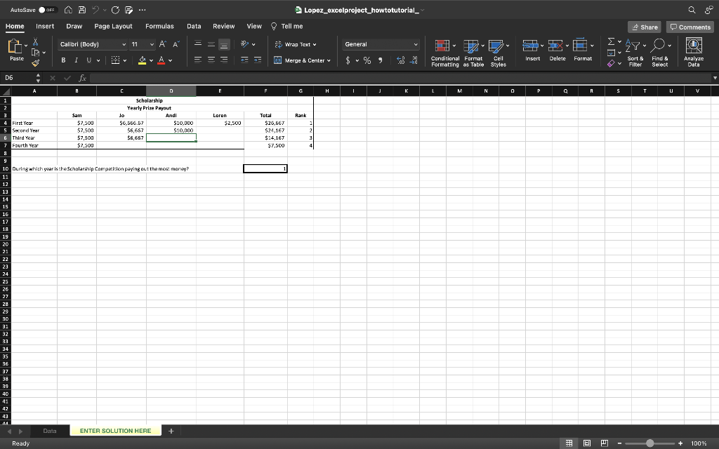
To determine during which year the scholarship competition is paying out the most money we can look ...
Get Instant Access to Expert-Tailored Solutions
See step-by-step solutions with expert insights and AI powered tools for academic success
Step: 2

Step: 3
Ace Your Homework with AI
Get the answers you need in no time with our AI-driven, step-by-step assistance
Get Started
Curriculum Alignment A Facilitators Developing Aligning And Auditing
Authors: Betty E. Steffy-English, Fenwick W. English
1st Edition
0803968485, 978-0803968486