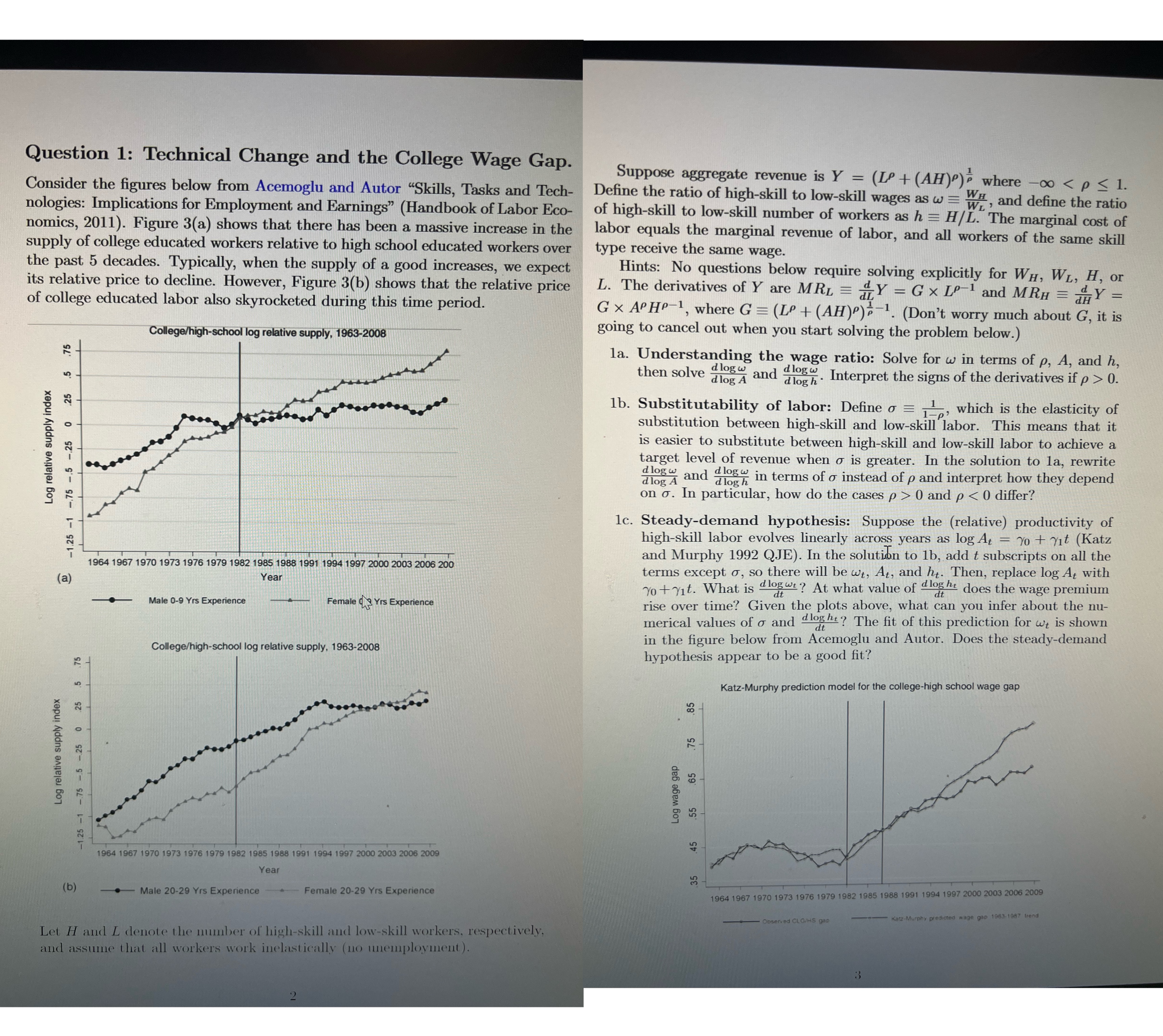
(b) Question 1: Technical Change and the College Wage Gap. Consider the figures below from Acemoglu and Autor "Skills, Tasks and Tech- nologies: Implications for Employment and Earnings" (Handbook of Labor Eco- nomics, 2011). Figure 3(a) shows that there has been a massive increase in the supply of college educated workers relative to high school educated workers over the past 5 decades. Typically, when the supply of a good increases, we expect its relative price to decline. However, Figure 3(b) shows that the relative price of college educated labor also skyrocketed during this time period. .25 .5 .75 0 Log relative supply index -1.25 -1.75 -5.25 (a) T College/high-school log relative supply, 1963-2008 1964 1967 1970 1973 1976 1979 1982 1985 1988 1991 1994 1997 2000 2003 2006 200 Year Male 0-9 Yrs Experience Female Yrs Experience College/high-school log relative supply, 1963-2008 (LP + (AH)") where -00 < p < 1. WH Suppose aggregate revenue is Y = Define the ratio of high-skill to low-skill wages as w=W, and define the ratio of high-skill to low-skill number of workers as h = H/L. The marginal cost of labor equals the marginal revenue of labor, and all workers of the same skill type receive the same wage. dH Hints: No questions below require solving explicitly for WH, WL, H, or L. The derivatives of Y are MRL = Y = G x LP-1 and MRH = Y = GX APHP-1, where G = (LP + (AH))-1. (Don't worry much about G, it is going to cancel out when you start solving the problem below.) 1a. Understanding the wage ratio: Solve for w in terms of p, A, and h, then solve dlog w dlogh Interpret the signs of the derivatives if p > 0. d log A and d log w 1b. Substitutability of labor: Define = 11, which is the elasticity of substitution between high-skill and low-skill labor. This means that it is easier to substitute between high-skill and low-skill labor to achieve a target level of revenue when is greater. In the solution to la, rewrite d log w and d log w in terms of instead of p and interpret how they depend dlog A on . In particular, how do the cases p > 0 and p < 0 differ? d log h 1c. Steady-demand hypothesis: Suppose the (relative) productivity of high-skill labor evolves linearly across years as log At = Yo + Yit (Katz and Murphy 1992 QJE). In the solution to 1b, add t subscripts on all the terms except , so there will be wt, At, and ht. Then, replace log At with Yo+yit. What is dogt? At what value of loght does the wage premium rise over time? Given the plots above, what can you infer about the nu- merical values of and d loght? The fit of this prediction for wt is shown in the figure below from Acemoglu and Autor. Does the steady-demand dt dt hypothesis appear to be a good fit? dt Katz-Murphy prediction model for the college-high school wage gap Log relative supply index -1.25 -1 -75 -5 -25 0 25 .5 75 Year Male 20-29 Yrs Experience 1964 1967 1970 1973 1976 1979 1982 1985 1988 1991 1994 1997 2000 2003 2006 2009 Female 20-29 Yrs Experience T Let H and L denote the number of high-skill and low-skill workers, respectively, and assume that all workers work inelastically (no unemployment). 2 Log wage gap 55 .65 .75 55 35 .45 45 .85 1964 1967 1970 1973 1976 1979 1982 1985 1988 1991 1994 1997 2000 2003 2006 2009 Observed CLG/HS gap Katz-Murphy predicted wage gap 1983-1987 trend 3