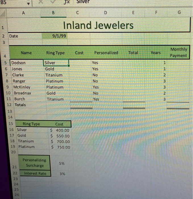
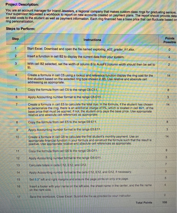
B5 Silver B D E E LL G 1 1 Inland Jewelers 9/1/99 2 Date 3 Ring Type Cost Personalized Total Years Monthly Payment 4 1 1 1 6 Name 4 5 Dodson Jones 7 Clarke 8 Ranger 9 McKinley 10 Broadnax 11 Burch 12 Totals Silver Gold Titanium Platinum Platinum Gold Titanium Yes Yes No No Yes No Yes NW WN 3 13 14 Cost 15 Ring Type 16 Silver 17 Gold 18 Titanium 19 Platinum 20 $ 400.00 $ 550.00 $ 700.00 $ 750.00 Personalizing Surcharge 5% 21 Interest Rate 3% 22 23 24 25 26 Project Description: You are an account manager for Inland Jewelers, a regional company that makes custom class rings for graduating seniors. Your supervisor requested a workbook to report on new accounts created on payment plans. The report should provide deta on total costs to the student as well as payment information. Each ring financed has a base price that can fluctuate based on ring personalization Steps to Perform: Step Instructions Points Possible 1 0 2 Start Excel. Download and open the file named exploring_e02_grader_h1.xlsx Insert a function in cell B2 to display the current date from your system. With cell B2 selected, set the width of column B to AutoFit (column width should then be set to 4. GS 2 9). 14 5 8 6 3 7 14 8 8 Create a formula in cell C5 using a lookup and reference function display the ring cost for the first student based on the selected ring type chosen in B5. Use relative and absolute cell addressing as appropriate. Copy the formula from cell C5 to the range C6:C11. Apply Accounting number format to the range C5:011. Create a formula in cell E5 to calculate the total due. In the formula, if the student has chosen to personalize the ring, there is an additional charge of 5%, which is located in cell B21, of the base price that must be applied; if not, the student only pays the base price. Use appropriate relative and absolute cell references as appropriate. Copy the formula from cell E5 to the range E6:E11. Apply Accounting number format to the range E5:E11. Create a formula in coll G5 to calculate the first student's monthly payment. Use an appropriate financial function in your formula and construct the formula such that the result is positive. Use appropriate relative and absolute cell references as appropriate. Copy tho formula from cells to the range G8:G11. Apply Accounting number format to the range 65:611. Calculate totals in cells C12, E12, and G12 Apply Accounting number format to the colls C12, E12, and G12, if necessary 9 10 14 11 12 3 13 7 14 3 5 15 Set 0.3" left and right margins and ensure the page prints on only one pago. Insert a footer with your name on the left side, the shoot name in the center, and the file name on the right sido 4 16 0 17 Save the workbook. Close Excel. Submit the fie as directed by your instructor Total Points 100