Begin the exercise by opening the file named Chapter 4 DA Exercise 2. Questions that are preceded with the lettersKOindicate you must only use your keyboard and not your mouse to execute the required skill.

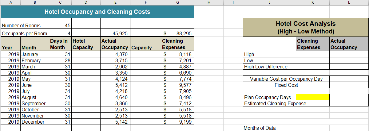
1. Enter a function in cell E3 that shows the total of adding the values in the range E5:E16. Use the output of this function to audit the data versus what was provided in the description of this exercise.
2. Enter a function in cell G3 that shows the total of adding the values in the range G5:G16. Use the output of this function to audit the data versus what was stated in the description of this exercise.
3. Enter a function in cell K17 that will count the number of months in the range B5:B17. Since the data in the worksheet should be for one year, verify that the output of the function makes sense. Also note that one blank cell, B17, is included in this range.
4. Enter a formula in cell D5 to calculate the January capacity for the hotel. The capacity is calculated by multiplying the occupants per room (cell C3) by the number of rooms in the hotel (cell C2). This result is then multiplied by the number of days in the month (cell C5). Construct this formula so that relative referencing does not change cells C3 and C2 when the formula is pasted into other cell locations.
5. Copy the formula in cell D5 and paste it into the range D6:D16. Use a paste method that does not change the border line style in column D.
6. Enter a formula in cell F5 to calculate the occupancy rate of the hotel. The formula should divide the Actual Occupancy by the Hotel Capacity. Format your result to a percentage with two decimal places.
7. Copy cell F5 and paste it into the range F6:F16. Use a paste method that uses the number format applied to cell F5 but does not change the border style in column F.
8. Enter a function in cell K5 that shows the highest value for the Cleaning Expenses in the range G5:G16.
9. KOCopy the function in cell K5 and paste it into cell K6 so the range used in the function does not change. Then modify the function so the output shows the lowest value for the Cleaning Expenses in the range G5:G16.
10. Enter a function in cell L5 that shows the highest value for the Actual Occupancy in the range E5:E16.
11. Copy the function in cell L5 and paste it into cell L6 so the range used in the function does not change. Then modify the function so the output shows the lowest value in the Cleaning Expenses column.
12. Enter a formula in cell K7 that subtracts the lowest Cleaning Expenses value from the highest Cleaning Expenses value.
13. Copy cell K7 and paste it into cell L7 such that only the formula is pasted without any of the formats from cell K7.
14. Enter a formula in cell L9 that divides the Cleaning Expenses High Low Difference (cell K7) by the Actual Occupancy High Low Difference (cell L7). The output of this formula shows the variable cost per occupancy day portion of the cleaning expenses per month. As mentioned in the description for this exercise, the cleaning expense is a mixed cost, which means it is comprised of both a variable and fixed cost.
15. Enter a formula in cell L10 that calculates the fixed cost portion for the cleaning expenses per month. Since we have calculated the variable cost per occupancy day, we can use it to calculate the fixed expense. First calculate the total variable expense by multiplying the variable expense per occupancy day in cell L9 by the High Actual Occupancy days in cell L5. Then, subtract this amount from the High Cleaning Expense in cell K5. Hint: You will have to put the calculation for the total variable expense in parentheses.
16. Enter the number 3500 in cell K12. Notice this cell is shaded yellow. Shading a cell is sometimes used to indicate a value that needs to be entered in order to produce an output. In this case, the value of 3,500 will be used to estimate the cleaning expenses.
17. Enter a formula in cell L13 that calculates the estimated cleaning expenses given the number that was entered into cell K12. Since the variable cost per occupancy day and the fixed cost is calculated in cells L9 and L10, these results can be used to estimate the cleaning expenses. The formula to estimate this mixed cost can be expressed as: Y=A+Bx where Y=Cleaning Expense, A is the fixed cost, B is the variable cost per occupancy day, and x is the number of occupancy days. The result of multiplying B times x is the total variable cost.
18. The output of the formula used to calculate the estimated cleaning expenses in cell L13 should be $6,900. Type the value 4800 in cell K12. You should see the cleaning estimate change to $8,720.
19. Type the following into the merged cell beginning with cell I16: Data added after row 16 is not included in this analysis. This alert will be used as part of a data internal control feature that will appear if additional data is added to the worksheet.
20. Change the font color in the merged cell beginning with I16 to white. It will appear as if the text has disappeared.
21. With the merged cell beginning with I16 still activated, click the Conditional Formatting button in the Home tab of the Ribbon.
22. Click the New Rule option from the dropdown menu. Set a conditional format rule based on the results of the following formula: =K17>12. If the value in cell K17 is greater than 12, then additional data has been added to the worksheet that will not be included in the outputs of the formulas and functions.
23. Select the bold and red font color for the conditional formats.
24. Type the word January in cell B17. This should trigger the conditional format and the alert should now be seen. This serves as a data internal control so the person using this worksheet will know that the formulas and functions need to be adjusted to account for the new data.
25. Save and close the workbook.