

Answered step by step
Verified Expert Solution
Question
1 Approved Answer
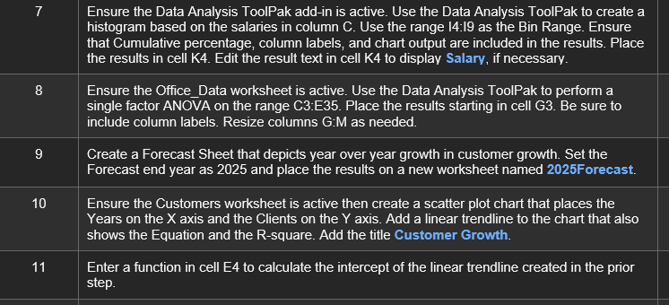
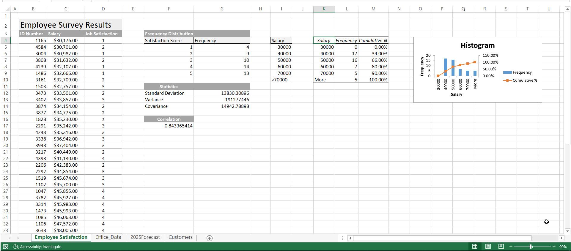
begin{tabular}{l|l} 7 & Ensure the Data Analysis ToolPak add-in is active. Use the Data Analysis ToolPak to create a end{tabular} histogram based on the salaries
Step by Step Solution
There are 3 Steps involved in it
Step: 1

Get Instant Access to Expert-Tailored Solutions
See step-by-step solutions with expert insights and AI powered tools for academic success
Step: 2

Step: 3
Ace Your Homework with AI
Get the answers you need in no time with our AI-driven, step-by-step assistance
Get Started
Privacy In Statistical Databases Cenex Sdc Project International Conference Psd 2006 Rome Italy December 2006 Proceedings Lncs 4302
Authors: Josep Domingo-Ferrer ,Luisa Franconi
2006th Edition
3540493301, 978-3540493303