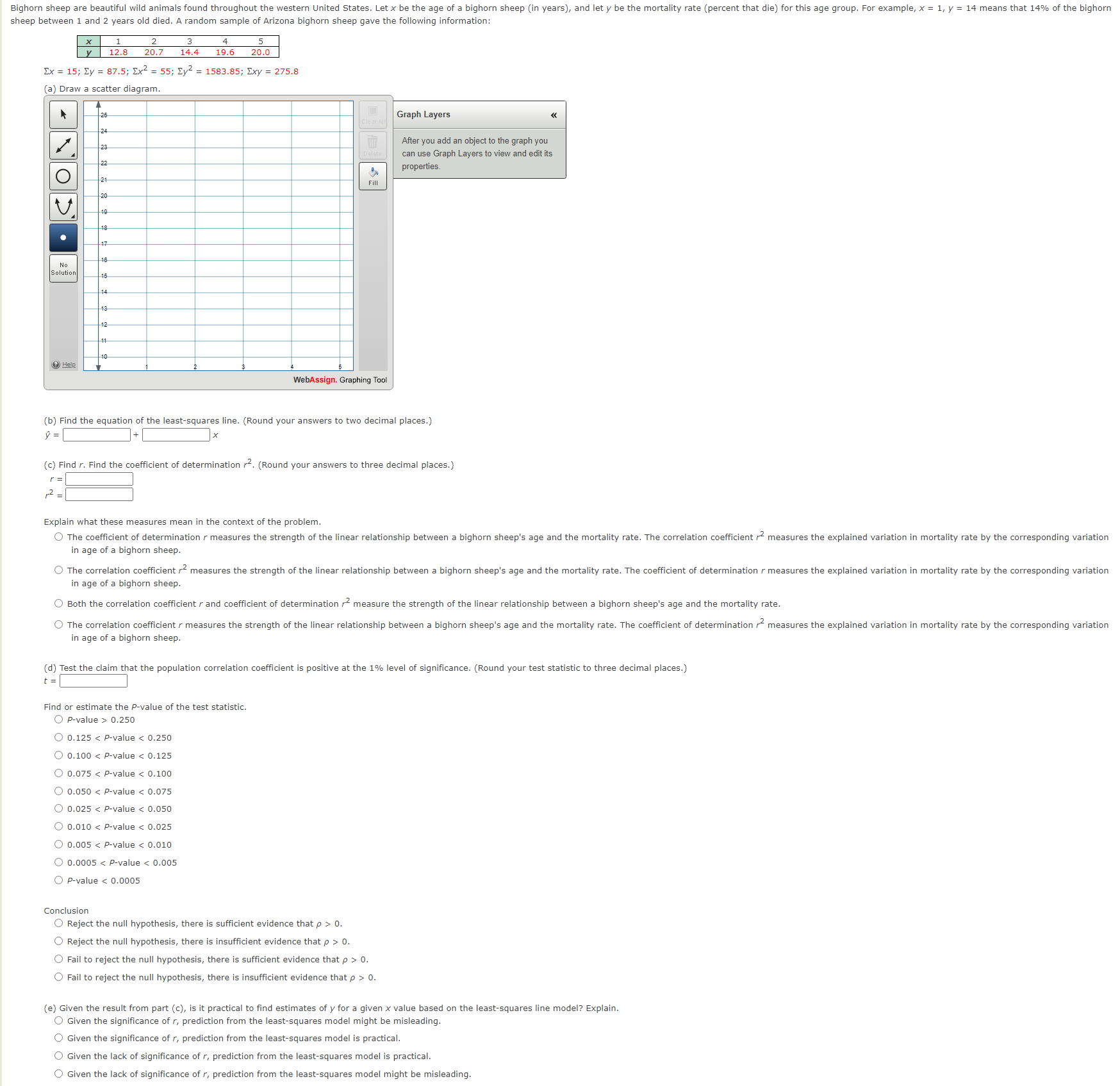
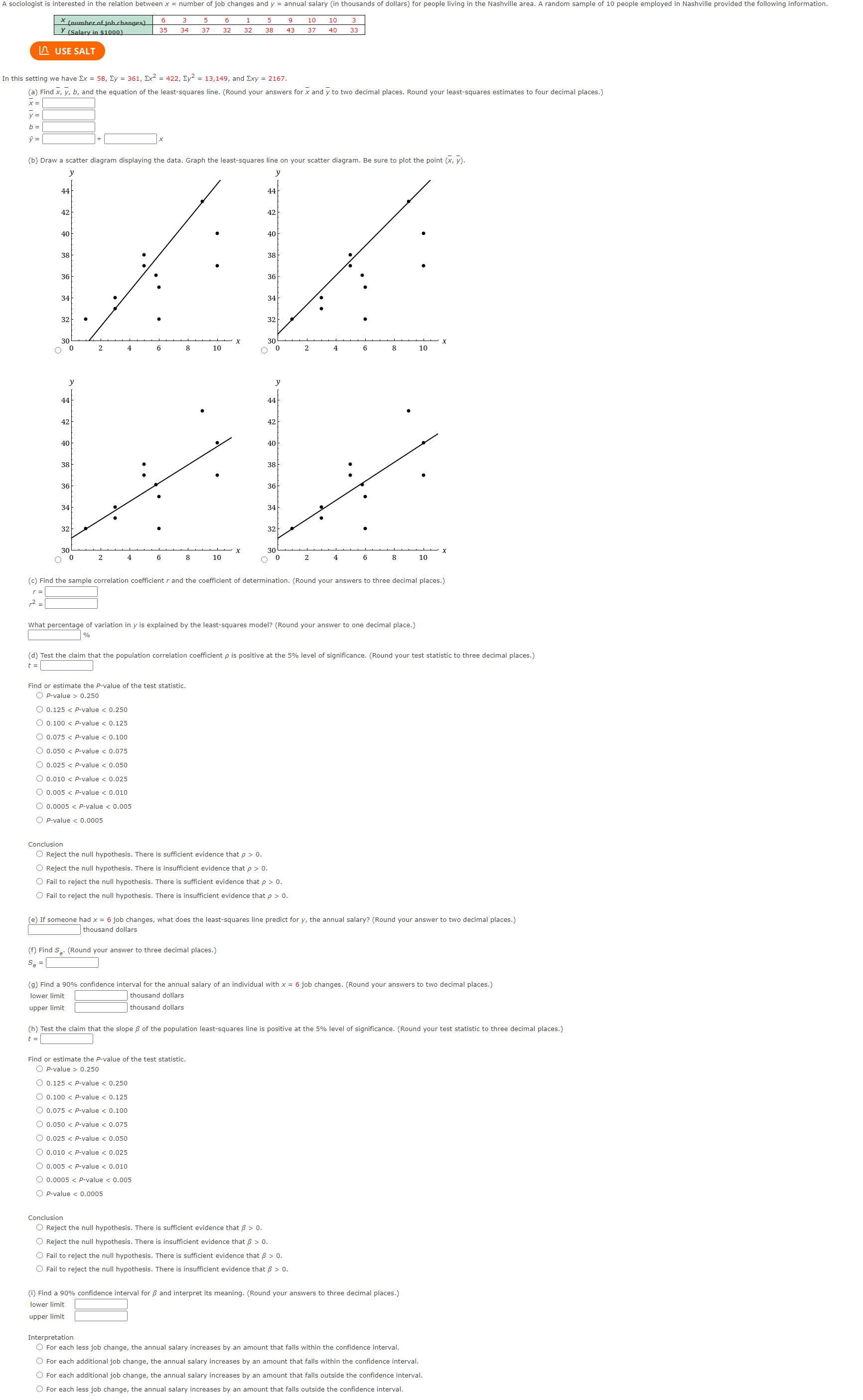
Bighorn sheep are beautiful wild animals found throughout the western United States. Let x be the age of a bighorn sheep (in years), and let y be the mortality rate (percent that die) for this age group. For example, x = 1, y = 14 means that 14% of the bighorn sheep between 1 and 2 years old died. A random sample of Arizona bighorn sheep gave the following information: x 1 2 3 4 5 y 12.8 20.7 14.4 19.6 20.0 Ex = 15; y = 87.5; Ex = 55; y = 1583.85; Exy = 275.8 (a) Draw a scatter diagram. 26 24 23 22 21 20 19 18 17 18 No Solution 15 14. 13 12 11 10 ? Help Fill WebAssign. Graphing Tool Graph Layers After you add an object to the graph you can use Graph Layers to view and edit its properties. (b) Find the equation of the least-squares line. (Round your answers to two decimal places.) = (c) Find r. Find the coefficient of determination r. (Round your answers to three decimal places.) r = 2 = Explain what these measures mean in the context of the problem. The coefficient of determination r measures the strength of the linear relationship between a bighorn sheep's age and the mortality rate. The correlation coefficient r measures the explained variation in mortality rate by the corresponding variation in age of a bighorn sheep. The correlation coefficient r measures the strength of the linear relationship between a bighorn sheep's age and the mortality rate. The coefficient of determination r measures the explained variation in mortality rate by the corresponding variation in age of a bighorn sheep. Both the correlation coefficient r and coefficient of determination measure the strength of the linear relationship between a bighorn sheep's age and the mortality rate. The correlation coefficient r measures the strength of the linear relationship between a bighorn sheep's age and the mortality rate. The coefficient of determination r measures the explained variation in mortality rate by the corresponding variation in age of a bighorn sheep. (d) Test the claim that the population correlation coefficient is positive at the 1% level of significance. (Round your test statistic to three decimal places.) t = Find or estimate the P-value of the test statistic. O P-value> 0.250 0.125 < P-value < 0.250 O 0.100 < P-value < 0.125 0.075 P-value < 0.100 0.050 < P-value < 0.075 0.025 P-value < 0.050 O 0.010 < P-value < 0.025 O 0.005 < P-value < 0.010 O 0.0005 < P-value < 0.005 OP-value < 0.0005 Conclusion Reject the null hypothesis, there is sufficient evidence that p > 0. Reject the null hypothesis, there is insufficient evidence that p > 0. Fail to reject the null hypothesis, there is sufficient evidence that p > 0. Fail to reject the null hypothesis, there is insufficient evidence that p > 0. (e) Given the result from part (c), is it practical to find estimates of y for a given x value based on the least-squares line model? Explain. Given the significance of r, prediction from the least-squares model might be misleading. Given the significance of r, prediction from the least-squares model is practical. Given the lack of significance of r, prediction from the least-squares model is practical. Given the lack of significance of r, prediction from the least-squares model might be misleading. A sociologist is interested in the relation between x = number of job changes and y = annual salary (in thousands of dollars) for people living in the Nashville area. A random sample of 10 people employed in Nashville provided the following information. (number of joh changes) 6 3 5 6 1 5 9 10 10 3 35 34 37 32 32 38 43 37 40 33 (Salary in $1000). USE SALT In this setting we have x = 58, y = 361, x = 422, y = 13,149, and 2xy = 2167. (a) Find x, y, b, and the equation of the least-squares line. (Round your answers for x and y to two decimal places. Round your least-squares estimates to four decimal places.) x = y = b= = X (b) Draw a scatter diagram displaying the data. Graph the least-squares line on your scatter diagram. Be sure to plot the point (x, y). y 44 42 40 38 36 34 32 y 44 42 40 38 36 34 32 30 x 30 X O 0 2 4 6 8 10 O 0 2 4 6 8 10 42 40 44 42 40 36 34 32 34 32 30 0 2 4 6 8 10 0 2 4 6 8 10 (c) Find the sample correlation coefficient r and the coefficient of determination. (Round your answers to three decimal places.) r = 2 = What percentage of variation in y is explained by the least-squares model? (Round your answer to one decimal place.) % (d) Test the claim that the population correlation coefficient p is positive at the 5% level of significance. (Round your test statistic to three decimal places.) t = Find or estimate the P-value of the test statistic. O P-value> 0.250 O 0.125 < P-value < 0.250 O 0.100 < P-value < 0.125 0.075 < P-value < 0.100 O 0.050 < P-value < 0.075 O 0.025 < P-value < 0.050 O 0.010 < P-value < 0.025 O 0.005 < P-value < 0.010 0.0005 < P-value < 0.005 P-value < 0.0005 Conclusion Reject the null hypothesis. There is sufficient evidence that p > 0. Reject the null hypothesis. There is insufficient evidence that p > 0. Fail to reject the null hypothesis. There is sufficient evidence that p > 0. Fail to reject the null hypothesis. There is insufficient evidence that p > 0. (e) If someone had x = 6 job changes, what does the least-squares line predict for y, the annual salary? (Round your answer to two decimal places.) thousand dollars (f) Find Se. (Round your answer to three decimal places.) Se = (g) Find a 90% confidence interval for the annual salary of an individual with x = 6 job changes. (Round your answers to two decimal places.) lower limit upper limit thousand dollars thousand dollars (h) Test the claim that the slope of the population least-squares line is positive at the 5% level of significance. (Round your test statistic to three decimal places.) t = Find or estimate the P-value of the test statistic. O P-value> 0.250 0.125 < P-value < 0.250 0.100 < P-value < 0.125 O 0.075 < P-value < 0.100 O 0.050 < P-value < 0.075 O 0.025 < P-value < 0.050 O 0.010 < P-value < 0.025 0.005 < P-value < 0.010 0.0005 < P-value < 0.005 O P-value < 0.0005 Conclusion Reject the null hypothesis. There is sufficient evidence that > 0. Reject the null hypothesis. There is insufficient evidence that > 0. Fail to reject the null hypothesis. There is sufficient evidence that > 0. Fail to reject the null hypothesis. There is insufficient evidence that > 0. (i) Find a 90% confidence interval for and interpret its meaning. (Round your answers to three decimal places.) lower limit upper limit Interpretation For each less job change, the annual salary increases by an amount that falls within the confidence interval. For each additional job change, the annual salary increases by an amount that falls within the confidence interval. For each additional job change, the annual salary increases by an amount that falls outside the confidence interval. For each less job change, the annual salary increases by an amount that falls outside the confidence interval.