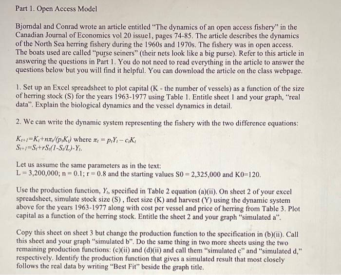
Bjorndal and Conrad wrote an article entitled "The dynamics of an open access fishery" in the Canadian Journal of Economics vol 20 issue1, pages 74-85. The article describes the dynamics of the North Sea herring fishery during the 1960 s and 1970s. The fishery was in open access. The boats used are called "purse seiners" (their nets look like a big purse). Refer to this article in answering the questions in Part 1 . You do not need to read everything in the article to answer the questions below but you will find it helpful. You can download the article on the class webpage. 1. Set up an Excel spreadsheet to plot capital ( K - the number of vessels) as a function of the size of herring stock (S) for the years 1963-1977 using Table 1. Entitle sheet 1 and your graph, "real data". Explain the biological dynamics and the vessel dynamics in detail. 2. We can write the dynamic system representing the fishery with the two difference equations: Kt+l=Kt+nl/(ptKi) where t=ptYtctKt St+1=St+rSt(1S/L)Yt Let us assume the same parameters as in the text: L=3,200,000;n=0.1;r=0.8 and the starting values S0=2,325,000 and K0=120. Use the production function, Yi, specified in Table 2 equation (a)(ii). On sheet 2 of your excel spreadsheet, simulate stock size (S) , fleet size (K) and harvest (Y) using the dynamic system above for the years 1963-1977 along with cost per vessel and price of herring from Table 3. Plot capital as a function of the herring stock. Entitle the sheet 2 and your graph "simulated a". Copy this sheet on sheet 3 but change the production function to the specification in (b)(ii). Call this sheet and your graph "simulated b". Do the same thing in two more sheets using the two remaining production functions: (c)(ii) and (d)(ii) and call them "simulated c" and "simulated d," respectively. Identify the production function that gives a simulated result that most closely follows the real data by writing "Best Fit" beside the graph title. Bjorndal and Conrad wrote an article entitled "The dynamics of an open access fishery" in the Canadian Journal of Economics vol 20 issue1, pages 74-85. The article describes the dynamics of the North Sea herring fishery during the 1960 s and 1970s. The fishery was in open access. The boats used are called "purse seiners" (their nets look like a big purse). Refer to this article in answering the questions in Part 1 . You do not need to read everything in the article to answer the questions below but you will find it helpful. You can download the article on the class webpage. 1. Set up an Excel spreadsheet to plot capital ( K - the number of vessels) as a function of the size of herring stock (S) for the years 1963-1977 using Table 1. Entitle sheet 1 and your graph, "real data". Explain the biological dynamics and the vessel dynamics in detail. 2. We can write the dynamic system representing the fishery with the two difference equations: Kt+l=Kt+nl/(ptKi) where t=ptYtctKt St+1=St+rSt(1S/L)Yt Let us assume the same parameters as in the text: L=3,200,000;n=0.1;r=0.8 and the starting values S0=2,325,000 and K0=120. Use the production function, Yi, specified in Table 2 equation (a)(ii). On sheet 2 of your excel spreadsheet, simulate stock size (S) , fleet size (K) and harvest (Y) using the dynamic system above for the years 1963-1977 along with cost per vessel and price of herring from Table 3. Plot capital as a function of the herring stock. Entitle the sheet 2 and your graph "simulated a". Copy this sheet on sheet 3 but change the production function to the specification in (b)(ii). Call this sheet and your graph "simulated b". Do the same thing in two more sheets using the two remaining production functions: (c)(ii) and (d)(ii) and call them "simulated c" and "simulated d," respectively. Identify the production function that gives a simulated result that most closely follows the real data by writing "Best Fit" beside the graph title


