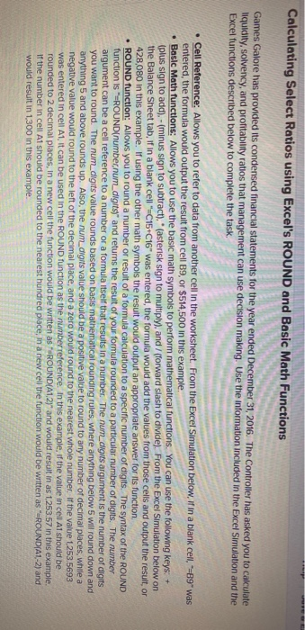
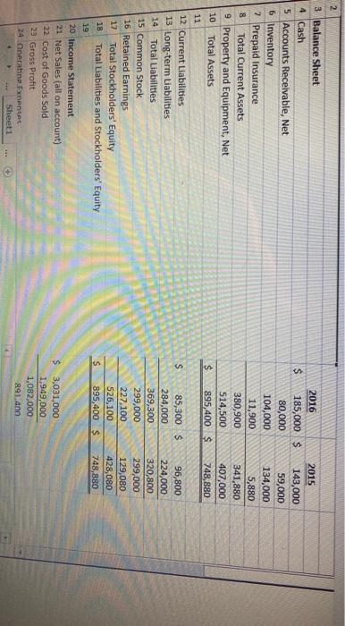
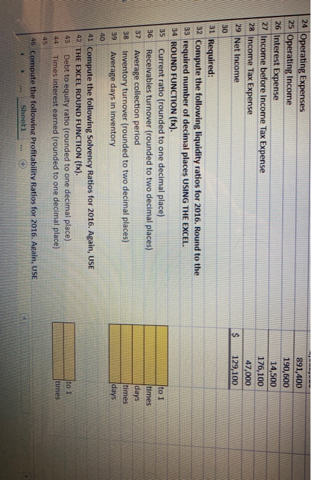
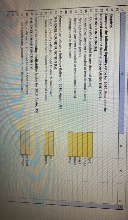
Calculating Select Ratios using Excel's ROUND and Basic Math Functions Games Galore has provided its condensed financial statements for the year ended December 31, 2016. The Controller has asked you to calculate liquidity, solvency, and profitability ratios that management can use decision making. Use the information included in the Excel Simulation and the Excel functions described below to complete the task. Cell Reference: Allows you to refer to data from another cell in the worksheet. From the Excel Simulation below, if in a blank cell, -89" was entered, the formula would output the result from cell B9, or $514,500 in this example, Basic Math functions: Allows you to use the basic math symbols to perform mathematical functions. You can use the following keys: + (plus sign to add).- (minus sign to subtract). * (asterisk sign to multiply), and / (forward slash to divide). From the Excel Simulation below on the Balance Sheet tab, if in a blank cell C15+C16" was entered, the formula would add the values from those cells and output the result, or 428,080 in this example. If using the other math symbols the result would output an appropriate answer for its function ROUND function: Allows you to round a number or result of a formula calculation to a specific number of digits. The syntax of the ROUND function is "-ROUND(number num_digits) and returns the result of your formula rounded to a particular number of digits. The number argument can be a cell reference to a number or a formula itself that results in a number. The num_digits argument is the number of digits you want to round. The num_digits value rounds based on basis mathematical rounding rules, where anything below 5 will round down and anything 5 and above rounds up. Also, the num_digits value should be a positive value to round to any number of decimal places, while a negative value would round to the left of the decimal place, and a zero would round to the nearest whole number. If the value 1253,5693 was entered in cell A1, it can be used in the ROUND Tunction as the number reference. In this example, if the value in cell A1 should be rounded to 2 decimal places, in a new cell the function would be written as 'ROUND(A1,27" and would result in as 1253.57 in this example, If the number in cell A1 should be rounded to the nearest hundred place in a new cell the function would be written as "=ROUND(A1-2) and would result in 1,300 in this example. 2 $ 2016 185,000 $ 80,000 104,000 11,900 380,900 514,500 895,400 $ 2015 143,000 59,000 134,000 5,880 341,880 407,000 748,880 $ $ 3 Balance Sheet 4 Cash 5 Accounts Receivable, Net 6 Inventory 7 Prepaid Insurance 8 Total Current Assets 9 Property and Equipment, Net 10 Total Assets 11 12 Current Liabilities 13 Long-term Liabilities 14 Total Liabilities 15 Common Stock 16 Retained Earnings 17 Total Stockholders' Equity 18 Total Liabilities and Stockholders' Equity 19 20 Income Statement 21 Net Sales (all on account) 22 Cost of Goods Sold 23 Gross Profit 24 Onerating Expenses Sheet1 85,300 $ 284,000 369,300 299,000 227,100 526,100 895,400 $ 96,800 224,000 320,800 299,000 129,080 428,080 748,880 $ $ 3,031,000 1,949,000 1,082,000 891.400 891,400 190,600 14,500 176,100 47,000 129, 100 $ 24 Operating Expenses 25 Operating Income 26 Interest Expense 27 Income before Income Tax Expense 28 Income Tax Expense 29 Net Income 30 31 Required: 32 Compute the following liquidity ratios for 2016. Round to the 33 required number of decimal places USING THE EXCEL. 34 ROUND FUNCTION (fx). 35 Current ratio (rounded to one decimal place) 36 Receivables turnover (rounded to two decimal places) 37 Average collection period 38 Inventory turnover (rounded to two decimal places) 39 Average days in inventory 40 41 Compute the following Solvency Ratios for 2016. Again, USE 42 THE EXCEL ROUND FUNCTION (fx). Debt to equity ratio (rounded to one decimal place) Times interest earned (rounded to one decimal place) 45 46 Compute the following Profitability Ratios for 2016. Again, USE Sheet1 to 1 times days times days 43 to 1 times 44 D 30 31 Required: 32 Compute the following liquidity ratios for 2016. Round to the 33 required number of decimal places USING THE EXCEL 34 ROUND FUNCTION (1x). 35 Current ratio (rounded to one decimal place) 36 Receivables turnover (rounded to two decimal places) 37 Average collection period 38 Inventory turnover (rounded to two decimal places) 39 Average days in inventory 40 41 Compute the following Solvency Ratios for 2016. Again, USE 42 THE EXCEL ROUND FUNCTION (fx). Debt to equity ratio (rounded to one decimal place) Times interest earned (rounded to one decimal place) to 1 times days times days 43 to 1 times 44 45 46 Compute the following profitability Ratios for 2016. Again, USE 47 THE EXCEL ROUND FUNCTION (fx). Net profit margin (rounded to one decimal place) Gross profit ratio (rounded to one decimal place) 48 percent percent 49 50 51 52