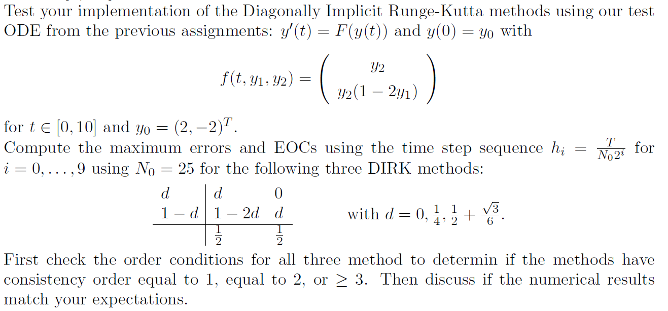
Can someone help me with the Runge-Kutta method, you are provided by the following code: import numpy as np from numpy import eye, array, exp, zeros, sqrt, cos, sin, pi from numpy.linalg import norm, inv from scipy.special import ellipj, ellipk from matplotlib import pyplot as plt

def dirk(f,Df, t0,y0, h, alpha,beta,gamma): # your code to compute y s = len(alpha) n = len(y0) k = np.zeros((s, n)) f0 = f(t0, y0) y = y0.copy().astype(float)

for i in range(s): ti = t0 + alpha[i]*h yi = y0 + h*sum([beta[i, l]*k[l, :] for l in range(i)]) if beta[i, i] == 0: k[i, :] = f(ti, yi) else: F = lambda d: d - f(ti, yi + h*beta[i, i]*d) DF = lambda d: np.eye(n) - h*beta[i, i]* Df(ti, yi + h*beta[i, i]*d) k[i, :] = newton(F, DF, f0, 1e-15, 1000)[0] y[:] += h*gamma[i]*k[i, :] return y def evolve(f, Df, t0, y0, h0, T, stepper): # initialize time and solution arrays n = int(T/h0) + 1 t = np.linspace(t0, T, n) y = np.zeros((n, len(y0))) y[0,:] = y0 # perform time integration for i in range(n-1): y[i+1,:] = stepper(f, Df, t[i], y[i,:], h0) return t, y def computeEocs(herr): m = len(herr) eocs = np.zeros(m - 1) for i in range(m-1): eocs[i] = np.log(herr[i+1,1]/herr[i,1])/ np.log(herr[i+1,0]/herr[i,0]) return eocs def crankNicholson(f, Df, t0, y0, h): F = lambda y: y-h/2 * f(t0+h, y) - (y0+h/2*f(t0, y0)) DF = lambda y: np.eye(len(y0)) - h/2 * Df(t0+h, y) y,n = newton(F, DF, y0, h*h*1e-5, 1000) assert n

def compareErrors(results): # columns of table simul = list(results.keys()) columns=['h'] + [s for n in simul for s in [f'{n}-error', f'{n}-eoc']] # values in tablea keys = {columns[0]: results[simul[0]][:,0]} # all results are assumed to use the same sequence of h styles = {columns[0]: '{:.4e}'} for i, k in enumerate(simul): keys[columns[2*i+1]] = results[k][:,1] # errors styles[columns[2*i+1]] = '{:.6e}' keys[columns[2*i+2]] = results[k][:,2] # eocs styles[columns[2*i+2]] = '{:.3f}'

# generate table table = pd.DataFrame(keys, index=range(results[simul[0]].shape[0]), # all results must have the same shape columns=columns)

# format floating points for each column for jupyter output (does not work in pdf) display( table.style.format(styles) )

for i,k in enumerate(simul): plt.loglog(results[k][:,0],results[k][:,1],marker='o',label=k) plt.legend() plt.grid(True) plt.ylim([None, 10]) # Added in case some method really messes up so that one can still see the good ones plt.xlabel("step size h") plt.ylabel("Maximum error over time") plt.savefig("Q2_compareErr.pdf", format="pdf", bbox_inches="tight") # output to pdf for inclusing in tex document plt.show() res = {} #res["FE"] = experiment(forwardEuler, f,Df,T,Y, M=10,N0=25) #res["BE"] = experiment(backwardEuler, f,Df,T,Y, M=10,N0=25) #res["Q11"] = experiment(Q11, f,Df,T,Y, M=10,N0=25) #res["CN"] = experiment(crankNicholson, f,Df,T,Y, M=10,N0=25) d = 0 #DIRK = lambda t, y,h: dirk(f,Df, t, y, h, alpha, beta, gamma) res = experiment(dirk,alpha, beta, gamma) res["dirk"] = experiment() compareErrors(res) Can anyone modify the code to create a list of table and plot a graph to show the comparison of different ds?

Implement a function to performs one step of a general diagonally implicit Runge-Kutta method. The two vectors and matrix defining the DIRK should be passed in to the function and the function needs to work for vector valued ODEs. Once you have implemented a function of the form defy=dirk(f,Df,t0,y0,h, alpha, beta, gamma) you can define a stepper fixing alpha, beta, gamma which you can then use in your evolve method, e.g., given the vectors and matrix alphaCN , betaCN , gammaCN defining the Crank-Nicholson method (provided in the lecture handout) the stepper is CrankNicholson = lambda f,Df,t0,y0:dirk(f,Df,t0,y0,alphaCN, betaCN, gammaCN) The rest of your code should then work without change. You can test your code by comparing the results you get with your old steppers (forwardEuler, backwardEuler,Q11,crankNicholsor The errors should be (close to) identical. Test your implementation of the Diagonally Implicit Runge-Kutta methods using our test ODE from the previous assignments: y(t)=F(y(t)) and y(0)=y0 with f(t,y1,y2)=(y2y2(12y1)) for t[0,10] and y0=(2,2)T. Compute the maximum errors and EOCs using the time step sequence hi=N02iT for i=0,,9 using N0=25 for the following three DIRK methods: d1dd12d210d21withd=0,41,21+63. First check the order conditions for all three method to determin if the methods have consistency order equal to 1 , equal to 2 , or 3. Then discuss if the numerical results match your expectations