can you please post it step by step

please let me know if its clear now. and can you please show all the steps that would be really helpful.

is it better now??

that's all the information i have in question

refund it please

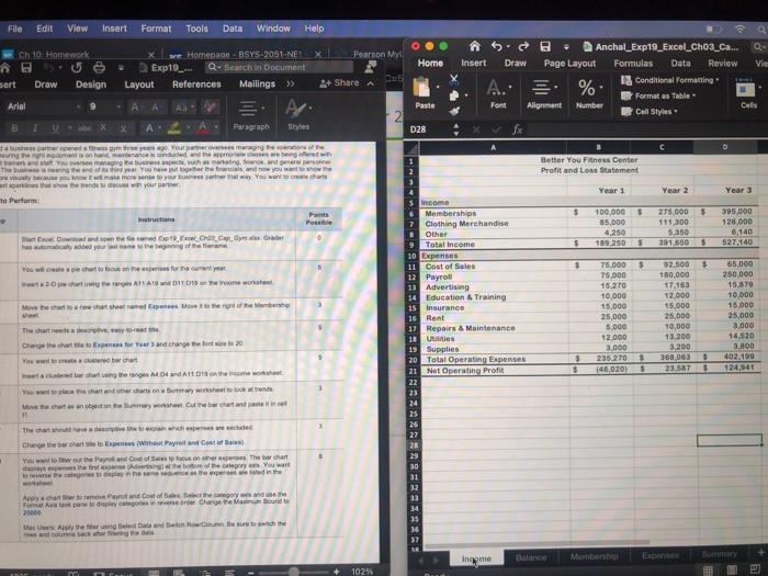
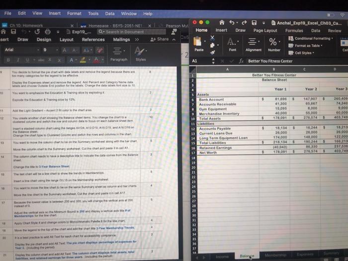
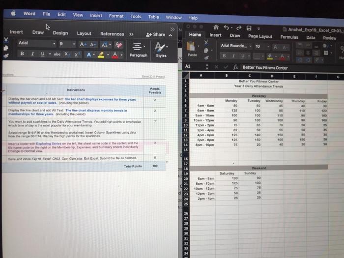
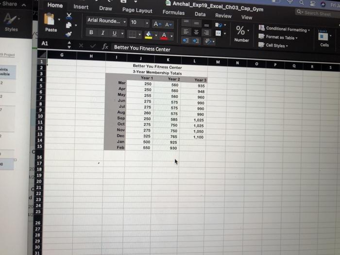
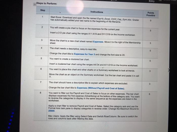
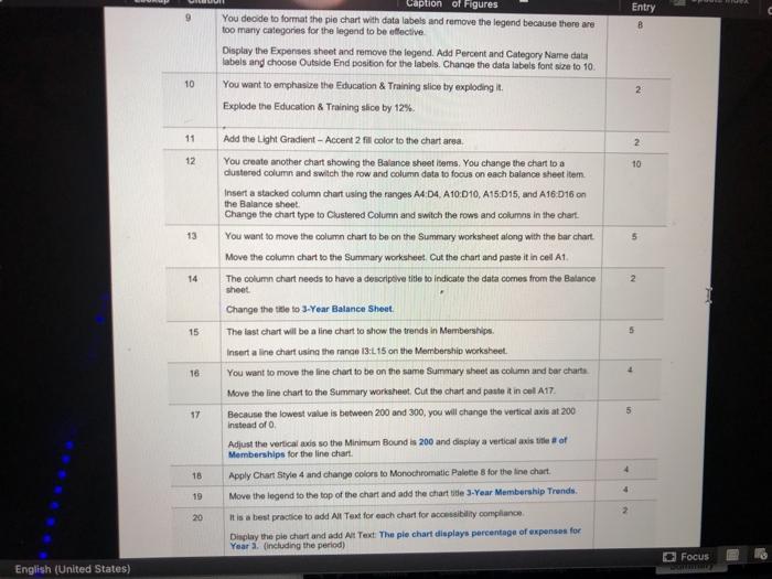
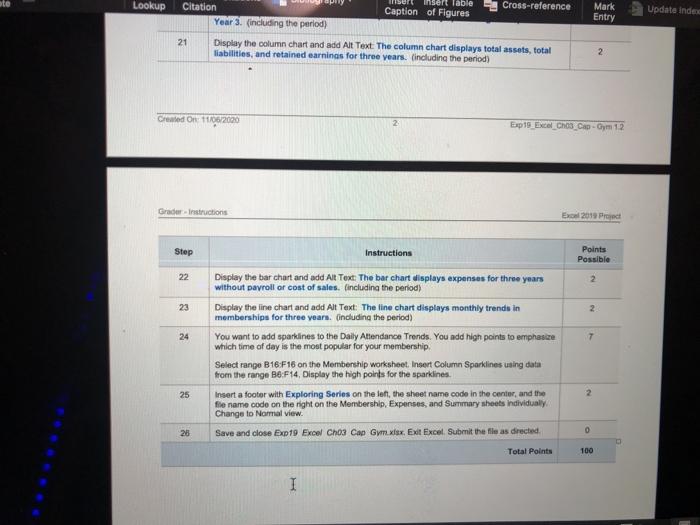
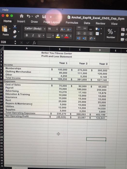
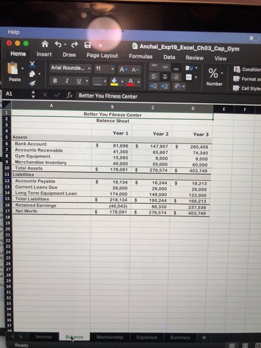
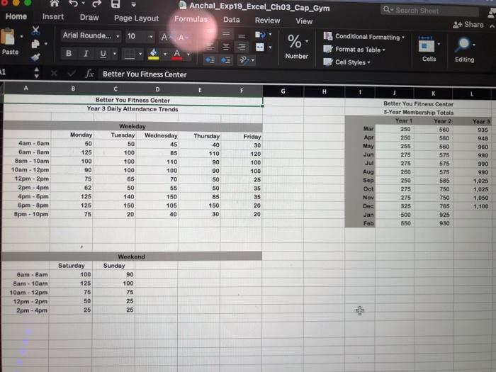
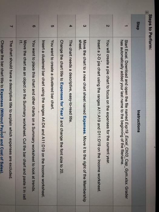
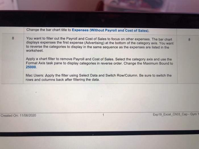
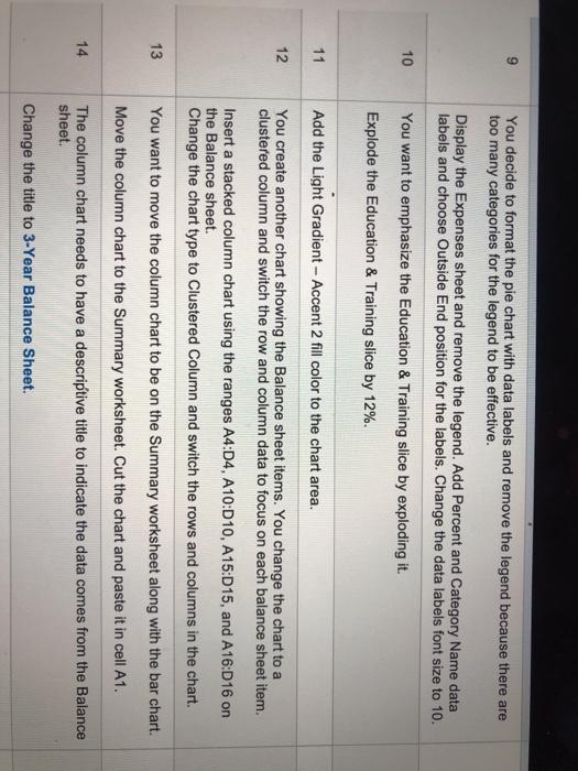
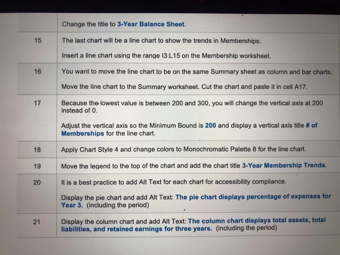
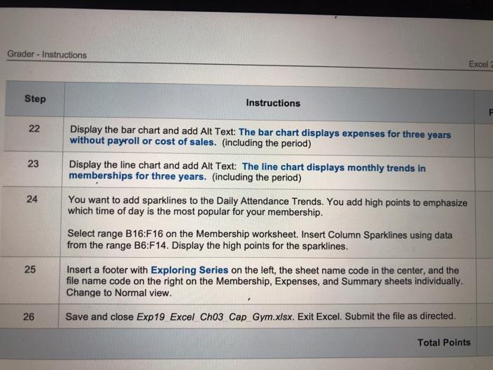
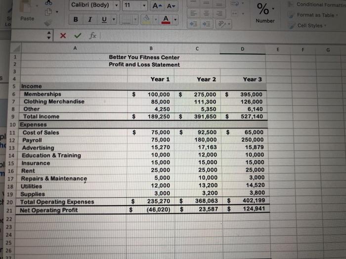
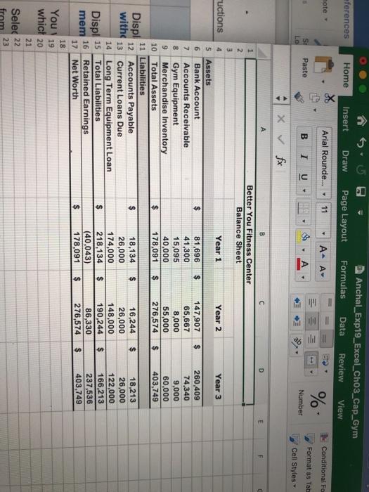
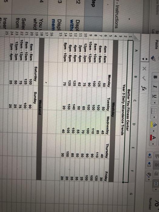
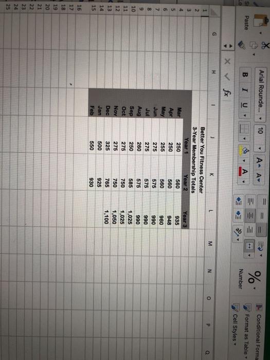
File Edit View Insert Format Tools Data Window Help Pearson Myl Home Ch.10: Homework B sert Drow Design Homepage - BSYS-2051-NE1 Exp19_ Q- Search in Document Layout References Mailings >> + Share 5. Anchal_Exp19_Excel_Cho3_Ca... Q- Insert Draw Page Layout Formulas Data Review Vie 1 Conditional Formatting A. % Format as Table Font Alignment Number Cells Cell Styles f Arial Paste 2 Paragraph Styles D28 Better You Fitness Center Profit and Loss Statement Year 1 Year 2 Year 3 ta benda yanging and weiger You managing the changer The goal Yadow you bow more anal way you want to showth your to Perform Pata Instruction Ponte Down med polymer amically beginning of the VOM $ $ $ 100,000 85,000 4,250 189.250 275.000 111.300 5250 301.650 395.000 128.000 0,140 527,140 $ $ $ $ $ 20 har AA19 Theme Me te arohad over the Members Income Membership 7 Clothing Merchandise 1 Other 9 Total income 10 Expenses 11 Cost of Sales 12 Payroll 1 Advertising 14 Education & Training 15 Insurance 16 Rent 17 Repair & Maintenance 10 Uits 19 Supplies 20 Total Operating Experts 21 Net Operating Profit 22 23 24 25 25 27 75.000 75.000 15,270 10,000 15,000 25,000 5.000 12.000 3.000 235270 146,020) 2.500 180,000 17,163 12.000 $5,000 25,000 10,000 13.200 3.200 368 063 23 58T 65,000 250.000 15.870 10.000 15,000 25,000 3.000 14,530 3.800 402,100 124,549 The charterova Change the hopes for your and change to 20 You webwch med behang there and A101 encome You with the many worstoso was not say what u behartan att 3 $ $ $ $ 1 3 E . Change rate to spenes (Without Payroll You want to the Pan Cost of the chart were the conce the perse wested in the 29 30 31 32 33 34 35 Apoyamond Goal Score Freevne Change in Beds 200 May the things and the best Ingane Balance Membership Expo 102% File Edit View Insert Format Tools Data Window Help Ch 10 Homework Pearson Myt Home Insert ere Homepage - BSYS 2051-NES Exp19_.. Q- Search in Document Layout References Mailings >> sert Draw Design 3+ Share A. 5. Anchal_Exp19_Excel_ch03_Ca... Draw Page Layout Formulas Data Review 1 Conditional Formatting Formatas Table Font Alignment Number Call Cell Styles fx Better You Fitness Center % . Arial 9 A Paste 2 Paragraph Styles A1 D 1 You hart will never end because there are margin to be by and move the percent Category Better You Fitness Center Balance Sheet Year 1 Year 2 Year) 10 7 You are medication Training by de Tuning by NMON $ 5 $1.500 41300 15.00 40,000 18.091 147,907 55,567 1,000 55,000 276.574 200,400 74.340 9,000 00 000 403.748 10 5 S $ A Great color to the charts You hart with whom you change the and whose che MDAD10 Att det Charge cartoon in the $ . $ 18.134 26,000 574.000 218.134 140,043 78.091 15,244 20.000 148.000 190 244 56330 278.574 5 Assets Bank Account Accounts Receivable Gym Equipment 9 Merchandise Inventory 10 Total Assets 11 Liabilities 12 Accounts Payabile 13 Current Loans Our 14 Long Term Equipment Loan 15 Total Liabities 16 Retained Earnings 17 Net Worth 18 19 20 21 22 23 24 25 26 27 13 $ 18.213 20,000 122.000 160,213 237530 403,40 . 5 14 2 More the course y Came channel Al The concert det er som om Chrow Balance 4 10 You were on the war mary and the Meet Day Out the channel! Betis 200 and you will change 200 17 At the sounds and 29 30 18 ply Changes to Moncho Palette for the chart da opet the stand the chararti Trends bod Touch Deprechart and Test The chantage of 2 33 34 35 34 21 Dy hecho Are The volum handel, Balance Member Word Fille Edit View Insert Format Tools Table Window Help Insert Draw Design Layout References >> >> 2+ Share A Home Insert Draw Anchal Exp19 Excel_cho_ Formulas Data Review Page Layout Arial A- A A Arial Rounde.... 10 * B I U obe XX Paragraph Styles Paste BI A1 Better You Fitness Center D Better You Fitness Center Year 3 Daily Attendance Trends 2 Instructions Points Possible 2 6 2 8 Wey Tuesday Wednesday 50 45 100 as 100 110 100 100 65 70 7 Day the bar art and and Alt Text The bar that displays expers for three year without payror cost of sales including the period Display the chart and Text The line chart displays monthly trunde in members for three years including the period You want to add sprinto the Day Atendance Trends. You did high posts which time of day is the most popular for your membership Select range 10 F 16 on Merbah woahet Imer Column Spordine ing data trometre 58. 14 Display the high port for the painen Insert for Exploring Series on the show in the cente teamebode on the right on the Map and Smily Change New Save and close to Brow Choa Cap Gym Excel Sutine the fie as directe Total Point Thursday 40 110 00 30 50 50 4ambam Gam-am Bam. 10am 10am-12pm 12pm-2pm 2pm pm 4pm pm Epm pm pm - 10pm Monday 50 125 100 90 75 62 125 125 75 9 10 11 12 13 14 15 Friday 30 120 100 100 25 35 35 20 20 110 105 150 2 150 30 0 100 16 17 18 19 20 21 22 d 23 24 25 Gam-Bam Bam 10am 10am-12pm 12pm-2pm 2pm. Apm Saturday 100 125 75 50 Weekend Sunday 30 100 75 25 25 26 27 28 29 30 31 32 33 - Share Home A a Fri Anchal_Exp19_Excel_Ch03_Cap_Gym Q- Search Sheet Insert Draw Page Layout Formulas Data Review Arial Rounde... 10 % 1 Conditional Formatting Formatas Table BIU Number Cells Cell Styles fx Better You Fitness Center View Styles Paste A1 H 1 S ints sible 2 Mar Apr May Jun Year 3 935 948 960 2 Better You Fitness Center 3-Year Membership Totals Year 1 Year 2 250 560 250 560 255 560 275 575 575 260 575 250 585 275 750 275 750 325 765 500 925 550 930 275 990 990 7 10 11 12 13 14 15 Aug Sep Oct Dec Jan Feb 990 1,025 1,025 1,050 1.100 2 0 16 17 2018 19 20 21 22 d 23 2024 25 26 27 28 29 30 31 Entry Steps to Perform: Step Instructions Points Possible 1 Start Excel. Download and open the file named Exp19 Excel_cho3_Cop_Gym.xlsx Grader has automatically added your last name to the beginning of the Siename 0 2 You will create a ple chart to focus on the expenses for the current year, Insert a 2-D ple chart using the ranges A11:A19 and 011:019 on the Income worksheet 5 3 3 4 5 5 5 3 Move the chart to a new chart sheet named Expenses. Move it to the right of the Membership sheet The chart needs a descriptive, easy-to-read title. Change the chart it to Expenses for Year 3 and change the font size to 20 You want to create a clustered bar chart. Insert a clustered bar chart using the ranges A4 D4 and A11:019 on the Income worksheet. You want to place this chart and other charts on a Summary worksheet to look at trends Move the chart as an object on the Summary worksheet. Cut the bar chart and paste it in cell 11 The chart should have a descriptive title to explain which expenses are excluded. Change the bar chart title to Expenses (Without Payroll and Cost of Sales) You want to filter out the Payroll and Cost of Sales to focus on other expenses. The bar chart displays expenses the first expense (Advertising) at the bottom of the category axis. You want to reverse the categories to display in the same sequence as the expenses are listed in the worksheet Apply a chart filter to remove Payroll and Cost of Sales Select the category axis and use the Format Axis task pane to display categories in reverse order. Change the Maximum Bound to 25000 7 3 Mac Users: Apply the filter using Select Data and Switch Row/Column. Be sure to switch the rows and columns back after filtering the data, Entry 9 Caption of Figures You decide to format the pie chart with data labels and remove the legend because there are too many categories for the legend to be effective Display the Expenses sheet and remove the legend. Add Percent and Category Name data labels and choose Outside End position for the labels Change the data labels font size to 10 You want to emphasize the Education & Training slice by exploding it. Explode the Education & Training sice by 12% 10 2. 11 2 12 10 13 5 14 2 15 5 Add the Light Gradient - Accent 2 fill color to the chart area. You create another chart showing the Balance sheet items. You change the chart to a clustered column and switch the row and column data to focus on each balance sheet item Insert a stacked column chart using the ranges A4:04. A10-010, A15.015, and A16D16 on the Balance sheet Change the chart type to Clustered Column and switch the rows and columns in the chart. You want to move the column chart to be on the Summary worksheet along with the bar chart Move the column chart to the Summary worksheet Cut the chart and paste it in cell A1 The column chart needs to have a descriptive title to indicate the data comes from the Balance sheet Change the title to 3-Year Balance Sheet The last chart will be a line chart to show the trends in Mermberships Insert a line chart using the ranon 13:1.15 on the Membership worksheet You want to move the line chart to be on the same Summary sheet as column and bar charts Move the line chart to the Summary worksheet Cut the chart and paste it in cel A17 Because the lowest value is butween 200 and 300, you will change the vertical axis at 200 Instead of Adjust the vertical ads so the Minimum Bound is 200 and display a vertical axis te of Membership for the line chart Apply Chart Style 4 and change colors to Monochromatic Palote for the line chart Move the legend to the top of the chart and add the chart title 3-Year Membership Trends It is a best practice to add A Text for each chart for accessibility compliance Display the pie chart and add Art Text. The ple chart displays percentage of expenses for Year (including the period) 4 18 17 5 18 4 19 2 20 Focus English (United States) Lookup Mark Entry Update Indee insert table Cross-reference Citation Caption of Figures Year 3. (including the period) 21 Display the column chart and add Alt Text: The column chart displays total assets, total liabilities, and retained earnings for three years, including the period) Created On 1700/2000 2 Ep 14 LXLC CHO CH GHI 12 Graderinstructions Exo 2019 Pro Step Instructions Points Possible 22 23 2 24 7 Display the bar chart and add Ait Text: The bar chart displays expenses for three years without payroll or cost of sales. including the period) Display the line chart and add Alt Text: The line chart displays monthly trends in membership for three years. (including the period) You want to add sparklines to the Daily Attendance Trends. You add high points to emphasize which time of day is the most popular for your membership Select range B16F16 on the Membership worksheet. Insert Column Sparklines using data from the range 86:F14, Display the high points for the sparklines. Insert a footer with Exploring Series on the lon, the sheet name code in the center, and the file name code on the right on the Membership Expenses, and Summary sheets individual Change to Nommal view Save and close Exp10 Excel Chou Cap Gym.xlsx. Exit Excel Submit the file as directed Total Points 25 2 26 0 100 1 Help Home Anchal_Exp19_Excel_Cho3_Cap_Gym Insert Draw Page Layout Formulas Data Review View Calibri (Body) 11 12C A- A+ % E BIU Number Paste F D28 A D E 1 Better You Fitness Center Profit and Loss Statement NMD Year 1 Year 2 Year 3 $ $ $ 100,000 85,000 4,250 189,250 275,000 111,300 5,350 391,650 395,000 126,000 6,140 527,140 $ $ $ $ $ $ 4 5 Income 6 Memberships 7 Clothing Merchandise 8 Other 9 Total Income 10 Expenses 11 Cost of Sales 12 Payroll 13 Advertising 14 Education & Training 15 Insurance 16 Rent 17 Repairs & Maintenance 18 Utilities 19 Supplies 20 Total Operating Expenses 21 Net Operating Profit 22 23 24 25 26 27 28 29 30 31 32 33 34 35 36 37 75,000 75,000 15,270 10,000 15,000 25,000 5,000 12,000 3,000 235,270 (46,020) 92,500 180,000 17,163 12,000 15,000 25,000 10,000 13,200 3,200 368,063 23,587 65,000 250,000 15,879 10,000 15,000 25,000 3,000 14,520 3,800 402,199 124,941 $ $ $ $ $ $ Help v Home Anchal_Exp19_Excel_Cho3_Cap_Gym Insert Draw Page Layout Formulas Data Review View Arial Rounde... 11 A- A- 12 Condition % Format as B I U Number Cell Style fx Better You Fitness Center Paste A1 D 1 2 3 Better You Fitness Center Balance Sheet Year 1 Year 2 Year 3 $ $ $ 81,696 41,300 15,095 40,000 178,091 147,907 65,667 8,000 55,000 276,574 260,409 74,340 9,000 60,000 403,749 $ $ $ 5 Assets Bank Account 7 Accounts Receivable 8 Gym Equipment 9 Merchandise Inventory 10 Total Assets 11 Liabilities 12 Accounts Payable 13 Current Loans Due 14 Long Term Equipment Loan 15 Total Liabilities 16 Retained Earnings 17 Net Worth 18 19 $ $ $ $ 18,134 26,000 174,000 218,134 (40,043) 178,091 16,244 26,000 148,000 190,244 86,330 276,574 $ $ 18,213 26,000 122,000 166,213 237.536 403,749 $ $ $ 21 22 23 24 25 26 27 28 29 30 31 32 33 34 35 36 37 2R Income Begance Membership Expenses Summary + Ready Paste Anchal_Exp19_Excel_Ch03_Cap_Gym Q- Search Sheet Home Insert Draw Page Layout Formulas Data Review View + Share Arial Rounde... 10 12 Conditional Formatting % Format as Table B I Number Cells Cell Styles Editing 11 Sx Better You Fitness Center D Better You Fitness Center Better You Fitness Center Year 3 Daily Attendance Trends 3-Year Membership Totals Yeart Year 2 Yoara Weekday Mar 250 560 935 Monday Tuesday Wednesday Thursday Friday Apr 250 560 948 4am - Bam 50 50 45 40 30 May 255 560 960 Gam-am 125 100 85 110 120 Jun 275 575 990 Bam - 10am 100 100 110 90 100 Jul 275 575 990 10am-12pm 90 100 100 90 100 Aug 260 575 990 12pm - 2pm 75 65 70 50 25 Sep 585 1,025 2pm - 4pm 62 50 55 50 35 275 750 1,025 4pm - 6pm 125 140 150 85 35 275 750 1,050 6pm - 8pm 125 150 105 20 Doc 325 765 1.100 Bpm - 10pm 75 20 40 30 20 Jan 500 925 Fab 550 930 250 Oct 150 Saturday 100 125 Gam-am Bam - 10am 10am-12pm 12pm-2pm 2pm - 4pm Weekend Sunday 90 100 75 25 25 75 50 25 Steps to Perform: Step Instructions Start Excel. Download and open the file named Exp19_Excel_Ch03_Cap_Gym.xlsx. Grader has automatically added your last name to the beginning of the filename. 2 You will create a pie chart to focus on the expenses for the current year. Insert a 2-D pie chart using the ranges A11:A19 and D11:019 on the Income worksheet. 3 Move the chart to a new chart sheet named Expenses. Move it to the right of the Membership sheet. 5 The chart needs a descriptive, easy-to-read title. Change the chart title to Expenses for Year 3 and change the font size to 20. You want to create a clustered bar chart. Insert a clustered bar chart using the ranges A4:04 and A11:019 on the Income worksheet. You want to place this chart and other charts on a Summary worksheet to look at trends. 6 Move the chart as an object on the Summary worksheet. Cut the bar chart and paste it in cell 11. 7 The chart should have a descriptive title to explain which expenses are excluded. Change the bar chart title to Expenses (Without Payroll and Cost of Sales). 8 8 Change the bar chart title to Expenses (Without Payroll and Cost of Sales), You want to filter out the Payroll and Cost of Sales to focus on other expenses. The bar chart displays expenses the first expense (Advertising) at the bottom of the category axis. You want to reverse the categories to display in the same sequence as the expenses are listed in the worksheet. Apply a chart filter to remove Payroll and Cost of Sales. Select the category axis and use the Format Axis task pane to display categories in reverse order. Change the Maximum Bound to 25000 Mac Users: Apply the filter using Select Data and Switch Row/Column. Be sure to switch the rows and columns back after filtering the data. Created On: 11/06/2020 1 Exp19_Excel_Cho3_Cap - Gym 1 You decide to format the pie chart with data labels and remove the legend because there are too many categories for the legend to be effective. Display the Expenses sheet and remove the legend. Add Percent and Category Name data labels and choose Outside End position for the labels. Change the data labels font size to 10. You want to emphasize the Education & Training slice by exploding it. Explode the Education & Training slice by 12%. 10 11 Add the Light Gradient - Accent 2 fill color to the chart area. 12 You create another chart showing the Balance sheet items. You change the chart to a clustered column and switch the row and column data to focus on each balance sheet item. Insert a stacked column chart using the ranges A4:D4, A10:D10, A15:D15, and A16:016 on the Balance sheet. Change the chart type to Clustered Column and switch the rows and columns in the chart. 13 You want to move the column chart to be on the Summary worksheet along with the bar chart. Move the column chart to the Summary worksheet. Cut the chart and paste it in cell A1. 14 The column chart needs to have a descriptive title to indicate the data comes from the Balance sheet. Change the title to 3-Year Balance Sheet. Change the title to 3-Year Balance Sheet. 15 The last chart will be a line chart to show the trends in Memberships. Insert a line chart using the range 13:L15 on the Membership worksheet. 16 17 You want to move the line chart to be on the same Summary sheet as column and bar charts. Move the line chart to the Summary worksheet. Cut the chart and paste it in cell A17. Because the lowest value is between 200 and 300, you will change the vertical axis at 200 instead of O. Adjust the vertical axis so the Minimum Bound is 200 and display a vertical axis title # of Memberships for the line chart. Apply Chart Style 4 and change colors to Monochromatic Palette 8 for the line chart. 18 19 Move the legend to the top of the chart and add the chart title 3-Year Membership Trends. 20 It is a best practice to add Alt Text for each chart for accessibility compliance. Display the pie chart and add Alt Text: The pie chart displays percentage of expenses for Year 3. (including the period) 21 Display the column chart and add Alt Text: The column chart displays total assets, total liabilities, and retained earnings for three years. (including the period) Grader - Instructions Excel 2 Step Instructions F 22 Display the bar chart and add Alt Text: The bar chart displays expenses for three years without payroll or cost of sales. (including the period) 23 24 Display the line chart and add Alt Text: The line chart displays monthly trends in memberships for three years. (including the period) You want to add sparklines to the Daily Attendance Trends. You add high points to emphasize which time of day is the most popular for your membership. Select range B16:F16 on the Membership worksheet. Insert Column Sparklines using data from the range B6:F14. Display the high points for the sparklines. 25 Insert a footer with Exploring Series on the left, the sheet name code in the center, and the file name code on the right on the Membership, Expenses, and Summary sheets individually. Change to Normal view. 26 Save and close Exp19 Excel Cho3 Cap Gym.xlsx. Exit Excel. Submit the file as directed. Total Points Calibri (Body) 11 . Conditional Formattin . % ili Format as Table Paste SI LO B T Number Cell Styles x fac A B E F G Better You Fitness Center Profit and Loss Statement Year 1 Year 2 Year 3 $ $ 100,000 85,000 4,250 189,250 275,000 111,300 5,350 391,650 395,000 126,000 6,140 527,140 $ $ $ $ $ 1 2 3 5 4 5 Income 6 Memberships 7 Clothing Merchandise 8 Other 9 Total Income 10 Expenses 11 Cost of Sales 12 Payroll ho 13 Advertising 14 Education & Training 15 Insurance 16 Rent 17 Repairs & Maintenance 18 Utilities 19 Supplies 20 Total Operating Expenses 21 Net Operating Profit $ 75,000 75,000 15,270 10,000 15,000 25,000 5,000 12,000 3,000 235,270 (46,020) 92,500 180,000 17,163 12,000 15,000 25,000 10,000 13,200 3,200 368,063 23,587 65,000 250,000 15,879 10,000 15,000 25,000 3,000 14,520 3,800 402,199 124,941 $ $ $ $ $ $ 1622 23 24 25 26 27 ferences Anchal_Exp19_Excel_ch03_Cap_Gym Home Insert Draw Page Layout Formulas Data Review View Arial Rounde... 11 A. A note = Conditional Fo % ill Format as Tab Paste SI LO B I U Number Cell Styles x fx B D E Better You Fitness Center Balance Sheet Year 1 Year 2 Year 3 $ $ $ 81,696 41,300 15,095 40,000 178,091 147,907 65,667 8,000 55,000 276,574 260,409 74,340 9,000 60,000 403,749 $ 1 2 3 ructions 4 5 Assets 6 Bank Account 7 Accounts Receivable B Gym Equipment 9 Merchandise Inventory 10 Total Assets 11 Liabilities Displ 12 Accounts Payable with 13 Current Loans Due 14 Long Term Equipment Loan Total Liabilities mem 16 Retained Earnings 17 Net Worth 18 You 19 $ $ $ $ 18,134 26,000 174,000 218,134 (40,043) 178,091 16,244 $ 26,000 148,000 190,244 $ 86,330 276,574 $ 18,213 26,000 122,000 166,213 237,536 403,749 $ $ Displ 15 $ $ whict 20 21 Sele 22 from 23 w Notes SI LO Paste I B IC A In M Me 70 Number X fx A B D Better You Fitness Center Year 3 Daily Attendance Trends - Instructions 1 2 3 4 5 6 7 Friday 30 120 100 tep 8 9 10 11 4am - 6am 6am - 8am 8am - 10am 10am-12pm 12pm - 2pm 2pm - 4pm 4pm - 6pm 6pm - 8pm 8pm - 10pm Monday 50 125 100 90 75 62 125 125 75 Weekday Tuesday Wednesday 50 45 100 85 100 110 100 100 65 70 50 55 140 150 150 105 20 40 Thursday 40 110 90 90 50 50 85 150 30 100 25 22 Displ 12 with 13 35 35 20 20 3 4 14 15 Displ mem 16 17 You 18 19 which 20 21 Selec 22 from 23 24 25 Inser 6am - Bam 8am - 10am 10am-12pm 12pm - 2pm 2pm - 4pm Saturday 100 125 75 50 Weekend Sunday 90 100 75 25 25 25 5 Arial Rounde... - 10 = II A- A+ Conditional Forma % inli M S Paste B U Format as Table Number 6 Cell Styles x v fx G H 1 L M N P 1 2 3 Mar 4 5 6 7 8 J Better You Fitness Center 3-Year Membership Totals Year 1 Year 2 250 560 250 560 255 560 275 575 275 575 260 575 250 585 275 750 275 750 325 765 500 925 550 930 Apr May Jun Jul Aug Sep Oct Nov Dec Jan Year 3 935 948 960 990 990 990 1,025 1,025 1,050 1,100 9 10 11 12 13 14 15 Feb 16 17 18 19 20 21 22 23 24 25 File Edit View Insert Format Tools Data Window Help Pearson Myl Home Ch.10: Homework B sert Drow Design Homepage - BSYS-2051-NE1 Exp19_ Q- Search in Document Layout References Mailings >> + Share 5. Anchal_Exp19_Excel_Cho3_Ca... Q- Insert Draw Page Layout Formulas Data Review Vie 1 Conditional Formatting A. % Format as Table Font Alignment Number Cells Cell Styles f Arial Paste 2 Paragraph Styles D28 Better You Fitness Center Profit and Loss Statement Year 1 Year 2 Year 3 ta benda yanging and weiger You managing the changer The goal Yadow you bow more anal way you want to showth your to Perform Pata Instruction Ponte Down med polymer amically beginning of the VOM $ $ $ 100,000 85,000 4,250 189.250 275.000 111.300 5250 301.650 395.000 128.000 0,140 527,140 $ $ $ $ $ 20 har AA19 Theme Me te arohad over the Members Income Membership 7 Clothing Merchandise 1 Other 9 Total income 10 Expenses 11 Cost of Sales 12 Payroll 1 Advertising 14 Education & Training 15 Insurance 16 Rent 17 Repair & Maintenance 10 Uits 19 Supplies 20 Total Operating Experts 21 Net Operating Profit 22 23 24 25 25 27 75.000 75.000 15,270 10,000 15,000 25,000 5.000 12.000 3.000 235270 146,020) 2.500 180,000 17,163 12.000 $5,000 25,000 10,000 13.200 3.200 368 063 23 58T 65,000 250.000 15.870 10.000 15,000 25,000 3.000 14,530 3.800 402,100 124,549 The charterova Change the hopes for your and change to 20 You webwch med behang there and A101 encome You with the many worstoso was not say what u behartan att 3 $ $ $ $ 1 3 E . Change rate to spenes (Without Payroll You want to the Pan Cost of the chart were the conce the perse wested in the 29 30 31 32 33 34 35 Apoyamond Goal Score Freevne Change in Beds 200 May the things and the best Ingane Balance Membership Expo 102% File Edit View Insert Format Tools Data Window Help Ch 10 Homework Pearson Myt Home Insert ere Homepage - BSYS 2051-NES Exp19_.. Q- Search in Document Layout References Mailings >> sert Draw Design 3+ Share A. 5. Anchal_Exp19_Excel_ch03_Ca... Draw Page Layout Formulas Data Review 1 Conditional Formatting Formatas Table Font Alignment Number Call Cell Styles fx Better You Fitness Center % . Arial 9 A Paste 2 Paragraph Styles A1 D 1 You hart will never end because there are margin to be by and move the percent Category Better You Fitness Center Balance Sheet Year 1 Year 2 Year) 10 7 You are medication Training by de Tuning by NMON $ 5 $1.500 41300 15.00 40,000 18.091 147,907 55,567 1,000 55,000 276.574 200,400 74.340 9,000 00 000 403.748 10 5 S $ A Great color to the charts You hart with whom you change the and whose che MDAD10 Att det Charge cartoon in the $ . $ 18.134 26,000 574.000 218.134 140,043 78.091 15,244 20.000 148.000 190 244 56330 278.574 5 Assets Bank Account Accounts Receivable Gym Equipment 9 Merchandise Inventory 10 Total Assets 11 Liabilities 12 Accounts Payabile 13 Current Loans Our 14 Long Term Equipment Loan 15 Total Liabities 16 Retained Earnings 17 Net Worth 18 19 20 21 22 23 24 25 26 27 13 $ 18.213 20,000 122.000 160,213 237530 403,40 . 5 14 2 More the course y Came channel Al The concert det er som om Chrow Balance 4 10 You were on the war mary and the Meet Day Out the channel! Betis 200 and you will change 200 17 At the sounds and 29 30 18 ply Changes to Moncho Palette for the chart da opet the stand the chararti Trends bod Touch Deprechart and Test The chantage of 2 33 34 35 34 21 Dy hecho Are The volum handel, Balance Member Word Fille Edit View Insert Format Tools Table Window Help Insert Draw Design Layout References >> >> 2+ Share A Home Insert Draw Anchal Exp19 Excel_cho_ Formulas Data Review Page Layout Arial A- A A Arial Rounde.... 10 * B I U obe XX Paragraph Styles Paste BI A1 Better You Fitness Center D Better You Fitness Center Year 3 Daily Attendance Trends 2 Instructions Points Possible 2 6 2 8 Wey Tuesday Wednesday 50 45 100 as 100 110 100 100 65 70 7 Day the bar art and and Alt Text The bar that displays expers for three year without payror cost of sales including the period Display the chart and Text The line chart displays monthly trunde in members for three years including the period You want to add sprinto the Day Atendance Trends. You did high posts which time of day is the most popular for your membership Select range 10 F 16 on Merbah woahet Imer Column Spordine ing data trometre 58. 14 Display the high port for the painen Insert for Exploring Series on the show in the cente teamebode on the right on the Map and Smily Change New Save and close to Brow Choa Cap Gym Excel Sutine the fie as directe Total Point Thursday 40 110 00 30 50 50 4ambam Gam-am Bam. 10am 10am-12pm 12pm-2pm 2pm pm 4pm pm Epm pm pm - 10pm Monday 50 125 100 90 75 62 125 125 75 9 10 11 12 13 14 15 Friday 30 120 100 100 25 35 35 20 20 110 105 150 2 150 30 0 100 16 17 18 19 20 21 22 d 23 24 25 Gam-Bam Bam 10am 10am-12pm 12pm-2pm 2pm. Apm Saturday 100 125 75 50 Weekend Sunday 30 100 75 25 25 26 27 28 29 30 31 32 33 - Share Home A a Fri Anchal_Exp19_Excel_Ch03_Cap_Gym Q- Search Sheet Insert Draw Page Layout Formulas Data Review Arial Rounde... 10 % 1 Conditional Formatting Formatas Table BIU Number Cells Cell Styles fx Better You Fitness Center View Styles Paste A1 H 1 S ints sible 2 Mar Apr May Jun Year 3 935 948 960 2 Better You Fitness Center 3-Year Membership Totals Year 1 Year 2 250 560 250 560 255 560 275 575 575 260 575 250 585 275 750 275 750 325 765 500 925 550 930 275 990 990 7 10 11 12 13 14 15 Aug Sep Oct Dec Jan Feb 990 1,025 1,025 1,050 1.100 2 0 16 17 2018 19 20 21 22 d 23 2024 25 26 27 28 29 30 31 Entry Steps to Perform: Step Instructions Points Possible 1 Start Excel. Download and open the file named Exp19 Excel_cho3_Cop_Gym.xlsx Grader has automatically added your last name to the beginning of the Siename 0 2 You will create a ple chart to focus on the expenses for the current year, Insert a 2-D ple chart using the ranges A11:A19 and 011:019 on the Income worksheet 5 3 3 4 5 5 5 3 Move the chart to a new chart sheet named Expenses. Move it to the right of the Membership sheet The chart needs a descriptive, easy-to-read title. Change the chart it to Expenses for Year 3 and change the font size to 20 You want to create a clustered bar chart. Insert a clustered bar chart using the ranges A4 D4 and A11:019 on the Income worksheet. You want to place this chart and other charts on a Summary worksheet to look at trends Move the chart as an object on the Summary worksheet. Cut the bar chart and paste it in cell 11 The chart should have a descriptive title to explain which expenses are excluded. Change the bar chart title to Expenses (Without Payroll and Cost of Sales) You want to filter out the Payroll and Cost of Sales to focus on other expenses. The bar chart displays expenses the first expense (Advertising) at the bottom of the category axis. You want to reverse the categories to display in the same sequence as the expenses are listed in the worksheet Apply a chart filter to remove Payroll and Cost of Sales Select the category axis and use the Format Axis task pane to display categories in reverse order. Change the Maximum Bound to 25000 7 3 Mac Users: Apply the filter using Select Data and Switch Row/Column. Be sure to switch the rows and columns back after filtering the data, Entry 9 Caption of Figures You decide to format the pie chart with data labels and remove the legend because there are too many categories for the legend to be effective Display the Expenses sheet and remove the legend. Add Percent and Category Name data labels and choose Outside End position for the labels Change the data labels font size to 10 You want to emphasize the Education & Training slice by exploding it. Explode the Education & Training sice by 12% 10 2. 11 2 12 10 13 5 14 2 15 5 Add the Light Gradient - Accent 2 fill color to the chart area. You create another chart showing the Balance sheet items. You change the chart to a clustered column and switch the row and column data to focus on each balance sheet item Insert a stacked column chart using the ranges A4:04. A10-010, A15.015, and A16D16 on the Balance sheet Change the chart type to Clustered Column and switch the rows and columns in the chart. You want to move the column chart to be on the Summary worksheet along with the bar chart Move the column chart to the Summary worksheet Cut the chart and paste it in cell A1 The column chart needs to have a descriptive title to indicate the data comes from the Balance sheet Change the title to 3-Year Balance Sheet The last chart will be a line chart to show the trends in Mermberships Insert a line chart using the ranon 13:1.15 on the Membership worksheet You want to move the line chart to be on the same Summary sheet as column and bar charts Move the line chart to the Summary worksheet Cut the chart and paste it in cel A17 Because the lowest value is butween 200 and 300, you will change the vertical axis at 200 Instead of Adjust the vertical ads so the Minimum Bound is 200 and display a vertical axis te of Membership for the line chart Apply Chart Style 4 and change colors to Monochromatic Palote for the line chart Move the legend to the top of the chart and add the chart title 3-Year Membership Trends It is a best practice to add A Text for each chart for accessibility compliance Display the pie chart and add Art Text. The ple chart displays percentage of expenses for Year (including the period) 4 18 17 5 18 4 19 2 20 Focus English (United States) Lookup Mark Entry Update Indee insert table Cross-reference Citation Caption of Figures Year 3. (including the period) 21 Display the column chart and add Alt Text: The column chart displays total assets, total liabilities, and retained earnings for three years, including the period) Created On 1700/2000 2 Ep 14 LXLC CHO CH GHI 12 Graderinstructions Exo 2019 Pro Step Instructions Points Possible 22 23 2 24 7 Display the bar chart and add Ait Text: The bar chart displays expenses for three years without payroll or cost of sales. including the period) Display the line chart and add Alt Text: The line chart displays monthly trends in membership for three years. (including the period) You want to add sparklines to the Daily Attendance Trends. You add high points to emphasize which time of day is the most popular for your membership Select range B16F16 on the Membership worksheet. Insert Column Sparklines using data from the range 86:F14, Display the high points for the sparklines. Insert a footer with Exploring Series on the lon, the sheet name code in the center, and the file name code on the right on the Membership Expenses, and Summary sheets individual Change to Nommal view Save and close Exp10 Excel Chou Cap Gym.xlsx. Exit Excel Submit the file as directed Total Points 25 2 26 0 100 1 Help Home Anchal_Exp19_Excel_Cho3_Cap_Gym Insert Draw Page Layout Formulas Data Review View Calibri (Body) 11 12C A- A+ % E BIU Number Paste F D28 A D E 1 Better You Fitness Center Profit and Loss Statement NMD Year 1 Year 2 Year 3 $ $ $ 100,000 85,000 4,250 189,250 275,000 111,300 5,350 391,650 395,000 126,000 6,140 527,140 $ $ $ $ $ $ 4 5 Income 6 Memberships 7 Clothing Merchandise 8 Other 9 Total Income 10 Expenses 11 Cost of Sales 12 Payroll 13 Advertising 14 Education & Training 15 Insurance 16 Rent 17 Repairs & Maintenance 18 Utilities 19 Supplies 20 Total Operating Expenses 21 Net Operating Profit 22 23 24 25 26 27 28 29 30 31 32 33 34 35 36 37 75,000 75,000 15,270 10,000 15,000 25,000 5,000 12,000 3,000 235,270 (46,020) 92,500 180,000 17,163 12,000 15,000 25,000 10,000 13,200 3,200 368,063 23,587 65,000 250,000 15,879 10,000 15,000 25,000 3,000 14,520 3,800 402,199 124,941 $ $ $ $ $ $ Help v Home Anchal_Exp19_Excel_Cho3_Cap_Gym Insert Draw Page Layout Formulas Data Review View Arial Rounde... 11 A- A- 12 Condition % Format as B I U Number Cell Style fx Better You Fitness Center Paste A1 D 1 2 3 Better You Fitness Center Balance Sheet Year 1 Year 2 Year 3 $ $ $ 81,696 41,300 15,095 40,000 178,091 147,907 65,667 8,000 55,000 276,574 260,409 74,340 9,000 60,000 403,749 $ $ $ 5 Assets Bank Account 7 Accounts Receivable 8 Gym Equipment 9 Merchandise Inventory 10 Total Assets 11 Liabilities 12 Accounts Payable 13 Current Loans Due 14 Long Term Equipment Loan 15 Total Liabilities 16 Retained Earnings 17 Net Worth 18 19 $ $ $ $ 18,134 26,000 174,000 218,134 (40,043) 178,091 16,244 26,000 148,000 190,244 86,330 276,574 $ $ 18,213 26,000 122,000 166,213 237.536 403,749 $ $ $ 21 22 23 24 25 26 27 28 29 30 31 32 33 34 35 36 37 2R Income Begance Membership Expenses Summary + Ready Paste Anchal_Exp19_Excel_Ch03_Cap_Gym Q- Search Sheet Home Insert Draw Page Layout Formulas Data Review View + Share Arial Rounde... 10 12 Conditional Formatting % Format as Table B I Number Cells Cell Styles Editing 11 Sx Better You Fitness Center D Better You Fitness Center Better You Fitness Center Year 3 Daily Attendance Trends 3-Year Membership Totals Yeart Year 2 Yoara Weekday Mar 250 560 935 Monday Tuesday Wednesday Thursday Friday Apr 250 560 948 4am - Bam 50 50 45 40 30 May 255 560 960 Gam-am 125 100 85 110 120 Jun 275 575 990 Bam - 10am 100 100 110 90 100 Jul 275 575 990 10am-12pm 90 100 100 90 100 Aug 260 575 990 12pm - 2pm 75 65 70 50 25 Sep 585 1,025 2pm - 4pm 62 50 55 50 35 275 750 1,025 4pm - 6pm 125 140 150 85 35 275 750 1,050 6pm - 8pm 125 150 105 20 Doc 325 765 1.100 Bpm - 10pm 75 20 40 30 20 Jan 500 925 Fab 550 930 250 Oct 150 Saturday 100 125 Gam-am Bam - 10am 10am-12pm 12pm-2pm 2pm - 4pm Weekend Sunday 90 100 75 25 25 75 50 25 Steps to Perform: Step Instructions Start Excel. Download and open the file named Exp19_Excel_Ch03_Cap_Gym.xlsx. Grader has automatically added your last name to the beginning of the filename. 2 You will create a pie chart to focus on the expenses for the current year. Insert a 2-D pie chart using the ranges A11:A19 and D11:019 on the Income worksheet. 3 Move the chart to a new chart sheet named Expenses. Move it to the right of the Membership sheet. 5 The chart needs a descriptive, easy-to-read title. Change the chart title to Expenses for Year 3 and change the font size to 20. You want to create a clustered bar chart. Insert a clustered bar chart using the ranges A4:04 and A11:019 on the Income worksheet. You want to place this chart and other charts on a Summary worksheet to look at trends. 6 Move the chart as an object on the Summary worksheet. Cut the bar chart and paste it in cell 11. 7 The chart should have a descriptive title to explain which expenses are excluded. Change the bar chart title to Expenses (Without Payroll and Cost of Sales). 8 8 Change the bar chart title to Expenses (Without Payroll and Cost of Sales), You want to filter out the Payroll and Cost of Sales to focus on other expenses. The bar chart displays expenses the first expense (Advertising) at the bottom of the category axis. You want to reverse the categories to display in the same sequence as the expenses are listed in the worksheet. Apply a chart filter to remove Payroll and Cost of Sales. Select the category axis and use the Format Axis task pane to display categories in reverse order. Change the Maximum Bound to 25000 Mac Users: Apply the filter using Select Data and Switch Row/Column. Be sure to switch the rows and columns back after filtering the data. Created On: 11/06/2020 1 Exp19_Excel_Cho3_Cap - Gym 1 You decide to format the pie chart with data labels and remove the legend because there are too many categories for the legend to be effective. Display the Expenses sheet and remove the legend. Add Percent and Category Name data labels and choose Outside End position for the labels. Change the data labels font size to 10. You want to emphasize the Education & Training slice by exploding it. Explode the Education & Training slice by 12%. 10 11 Add the Light Gradient - Accent 2 fill color to the chart area. 12 You create another chart showing the Balance sheet items. You change the chart to a clustered column and switch the row and column data to focus on each balance sheet item. Insert a stacked column chart using the ranges A4:D4, A10:D10, A15:D15, and A16:016 on the Balance sheet. Change the chart type to Clustered Column and switch the rows and columns in the chart. 13 You want to move the column chart to be on the Summary worksheet along with the bar chart. Move the column chart to the Summary worksheet. Cut the chart and paste it in cell A1. 14 The column chart needs to have a descriptive title to indicate the data comes from the Balance sheet. Change the title to 3-Year Balance Sheet. Change the title to 3-Year Balance Sheet. 15 The last chart will be a line chart to show the trends in Memberships. Insert a line chart using the range 13:L15 on the Membership worksheet. 16 17 You want to move the line chart to be on the same Summary sheet as column and bar charts. Move the line chart to the Summary worksheet. Cut the chart and paste it in cell A17. Because the lowest value is between 200 and 300, you will change the vertical axis at 200 instead of O. Adjust the vertical axis so the Minimum Bound is 200 and display a vertical axis title # of Memberships for the line chart. Apply Chart Style 4 and change colors to Monochromatic Palette 8 for the line chart. 18 19 Move the legend to the top of the chart and add the chart title 3-Year Membership Trends. 20 It is a best practice to add Alt Text for each chart for accessibility compliance. Display the pie chart and add Alt Text: The pie chart displays percentage of expenses for Year 3. (including the period) 21 Display the column chart and add Alt Text: The column chart displays total assets, total liabilities, and retained earnings for three years. (including the period) Grader - Instructions Excel 2 Step Instructions F 22 Display the bar chart and add Alt Text: The bar chart displays expenses for three years without payroll or cost of sales. (including the period) 23 24 Display the line chart and add Alt Text: The line chart displays monthly trends in memberships for three years. (including the period) You want to add sparklines to the Daily Attendance Trends. You add high points to emphasize which time of day is the most popular for your membership. Select range B16:F16 on the Membership worksheet. Insert Column Sparklines using data from the range B6:F14. Display the high points for the sparklines. 25 Insert a footer with Exploring Series on the left, the sheet name code in the center, and the file name code on the right on the Membership, Expenses, and Summary sheets individually. Change to Normal view. 26 Save and close Exp19 Excel Cho3 Cap Gym.xlsx. Exit Excel. Submit the file as directed. Total Points Calibri (Body) 11 . Conditional Formattin . % ili Format as Table Paste SI LO B T Number Cell Styles x fac A B E F G Better You Fitness Center Profit and Loss Statement Year 1 Year 2 Year 3 $ $ 100,000 85,000 4,250 189,250 275,000 111,300 5,350 391,650 395,000 126,000 6,140 527,140 $ $ $ $ $ 1 2 3 5 4 5 Income 6 Memberships 7 Clothing Merchandise 8 Other 9 Total Income 10 Expenses 11 Cost of Sales 12 Payroll ho 13 Advertising 14 Education & Training 15 Insurance 16 Rent 17 Repairs & Maintenance 18 Utilities 19 Supplies 20 Total Operating Expenses 21 Net Operating Profit $ 75,000 75,000 15,270 10,000 15,000 25,000 5,000 12,000 3,000 235,270 (46,020) 92,500 180,000 17,163 12,000 15,000 25,000 10,000 13,200 3,200 368,063 23,587 65,000 250,000 15,879 10,000 15,000 25,000 3,000 14,520 3,800 402,199 124,941 $ $ $ $ $ $ 1622 23 24 25 26 27 ferences Anchal_Exp19_Excel_ch03_Cap_Gym Home Insert Draw Page Layout Formulas Data Review View Arial Rounde... 11 A. A note = Conditional Fo % ill Format as Tab Paste SI LO B I U Number Cell Styles x fx B D E Better You Fitness Center Balance Sheet Year 1 Year 2 Year 3 $ $ $ 81,696 41,300 15,095 40,000 178,091 147,907 65,667 8,000 55,000 276,574 260,409 74,340 9,000 60,000 403,749 $ 1 2 3 ructions 4 5 Assets 6 Bank Account 7 Accounts Receivable B Gym Equipment 9 Merchandise Inventory 10 Total Assets 11 Liabilities Displ 12 Accounts Payable with 13 Current Loans Due 14 Long Term Equipment Loan Total Liabilities mem 16 Retained Earnings 17 Net Worth 18 You 19 $ $ $ $ 18,134 26,000 174,000 218,134 (40,043) 178,091 16,244 $ 26,000 148,000 190,244 $ 86,330 276,574 $ 18,213 26,000 122,000 166,213 237,536 403,749 $ $ Displ 15 $ $ whict 20 21 Sele 22 from 23 w Notes SI LO Paste I B IC A In M Me 70 Number X fx A B D Better You Fitness Center Year 3 Daily Attendance Trends - Instructions 1 2 3 4 5 6 7 Friday 30 120 100 tep 8 9 10 11 4am - 6am 6am - 8am 8am - 10am 10am-12pm 12pm - 2pm 2pm - 4pm 4pm - 6pm 6pm - 8pm 8pm - 10pm Monday 50 125 100 90 75 62 125 125 75 Weekday Tuesday Wednesday 50 45 100 85 100 110 100 100 65 70 50 55 140 150 150 105 20 40 Thursday 40 110 90 90 50 50 85 150 30 100 25 22 Displ 12 with 13 35 35 20 20 3 4 14 15 Displ mem 16 17 You 18 19 which 20 21 Selec 22 from 23 24 25 Inser 6am - Bam 8am - 10am 10am-12pm 12pm - 2pm 2pm - 4pm Saturday 100 125 75 50 Weekend Sunday 90 100 75 25 25 25 5 Arial Rounde... - 10 = II A- A+ Conditional Forma % inli M S Paste B U Format as Table Number 6 Cell Styles x v fx G H 1 L M N P 1 2 3 Mar 4 5 6 7 8 J Better You Fitness Center 3-Year Membership Totals Year 1 Year 2 250 560 250 560 255 560 275 575 275 575 260 575 250 585 275 750 275 750 325 765 500 925 550 930 Apr May Jun Jul Aug Sep Oct Nov Dec Jan Year 3 935 948 960 990 990 990 1,025 1,025 1,050 1,100 9 10 11 12 13 14 15 Feb 16 17 18 19 20 21 22 23 24 25