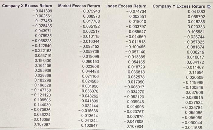
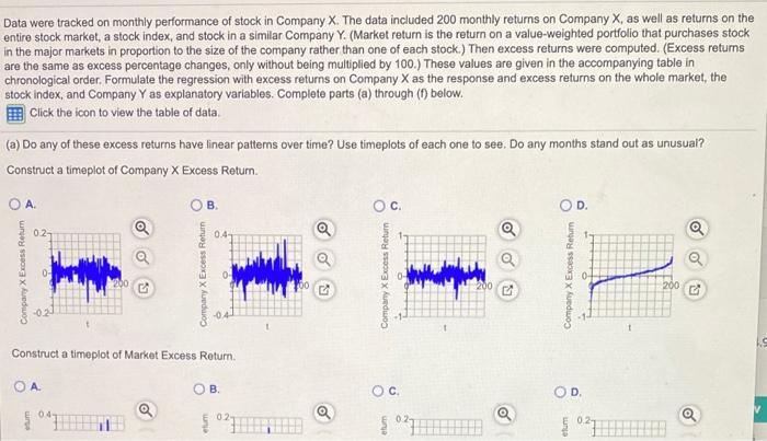
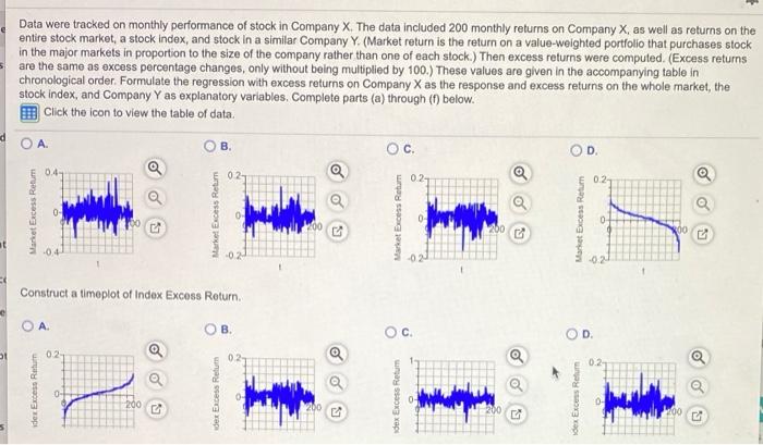
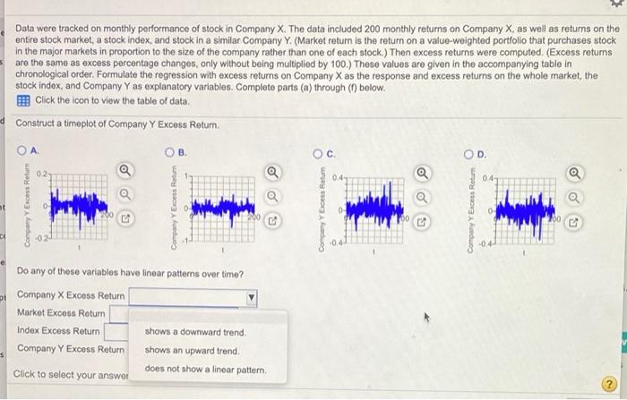
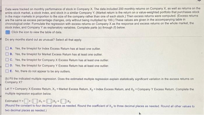
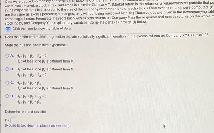
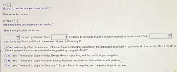
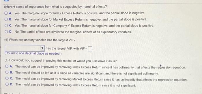
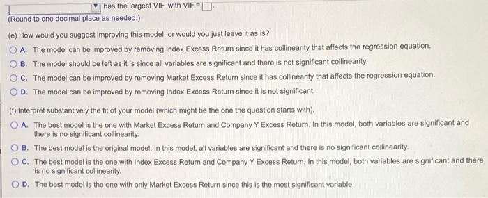
Company X Excess Return -0.041399 -0.002561 0.177450 -0.028485 0.043971 0.078935 -0.068223 -0.122640 -0.222163 0.053719 0.193430 0.164106 0.285939 0.028869 0.183296 -0.196528 -0.147758 -0.121120 0.109505 0.144030 -0.070636 0.036224 -0.016055 0.107097 Market Excess Return -0.075943 0.008973 0.017708 -0.035192 0.082517 -0.010115 -0.016044 -0.098152 -0.059738 -0.019099 0.060153 0.023608 0.044488 0.071106 0.024505 -0.001950 0.036378 -0.048262 0.041899 0.022144 -0.015636 0.013614 -0.041244 0.102947 Index Excess Return -0.074734 0.002551 0.018010 -0.033797 0.085547 -0.014669 -0.011818 -0.100465 -0.057140 -0.013385 0.054165 0.018729 0.036818 0.062578 0.017950 -0.005017 0.034270 -0.052120 0.039946 0.014996 -0.023757 0.007679 -0.047808 0.107904 Company Y Excess Return 0.041883 0.059702 0.015286 0.020333 0.105581 -0.026744 -0.057825 -0.081674 0.038219 -0.016017 0.084172 -0.011467 0.11694 0.020509 -0.119998 -0.100849 0.037606 -0.088915 0.037534 -0.035784 0.065085 -0.056059 -0.050044 -0.041585 Data were tracked on monthly performance of stock in Company X. The data included 200 monthly returns on Company X, as well as returns on the entire stock market, a stock index, and stock in a similar Company Y. (Market return is the return on a value-weighted portfolio that purchases stock in the major markets in proportion to the size of the company rather than one of each stock.) Then excess returns were computed. (Excess returns are the same as excess percentage changes, only without being multiplied by 100.) These values are given in the accompanying table in chronological order. Formulate the regression with excess returns on Company X as the response and excess returns on the whole market, the stock Index, and Company Y as explanatory variables. Complete parts (a) through (1) below. Click the icon to view the table of data. (a) Do any of these excess returns have linear patterns over time? Use timeplots of each one to see. Do any months stand out as unusual? Construct a timeplot of Company X Excess Return A O B o C. O 02 Q 0.4 a o o Company X Excess Retum Company X Excess Return Company X Excess Return Company X Excess Retur 200 200 Construct a timeplot of Market Excess Return . . , OD 02 Q 0.2- ? Data were tracked on monthly performance of stock in Company X. The data included 200 monthly returns on Company X, as well as returns on the entire stock market, a stock Index, and stock in a similar Company Y. (Market return is the return on a value-weighted portfolio that purchases stock in the major markets in proportion to the size of the company rather than one of each stock.) Then excess returns were computed. (Excess returns are the same as excess porcentage changes, only without being multiplied by 100.) These values are given in the accompanying table in chronological order. Formulate the regression with excess returns on Company X as the response and excess returns on the whole market, the stock index, and Company Y as explanatory variables. Complete parts (a) through (1) below. Click the icon to view the table of data. d A. OB OC. D 0.4- Q 02 Q 02- a 0.2 Market Excess Retum Market Excess Return Market Excess Rota Market Excess Retur 4 Construct a timeplot of Index Excess Return OA . . OD 31 021 02 Q 0 0.2 dex Excess Return dex Excess Retum OS dex Excess Retum ex Exco Return 200 Data were tracked on monthly performance of stock in Company X. The data included 200 monthly returns on Company X, as well as returns on the entire stock market, a stock index, and stock in a similar Company Y. (Market return is the return on a value-weighted portfolio that purchases stock in the major markets in proportion to the size of the company rather than one of each stock.) Then excess returns were computed. (Excess retums are the same as excess percentage changes, only without being multiplied by 100.) These values are given in the accompanying table in chronological order. Formulate the regression with excess returns on Company X as the response and excess returns on the whole market, the stock index, and Company Y as explanatory variables. Complete parts (a) through (1) below. Click the icon to view the table of data. Do any months stand out as unusual? Select all that apply. A. Yes, the timeplot for Index Excess Return has at least one outlier, B. Yes, the timoplot for Market Excess Return has at least one outlier. C. Yes, the timeplot for Company X Excess Return has at least one outlier. D. Yes, the timeplot for Company Y Excess Return has at least one outlier. E. No, there do not appear to be any outliers (b) Fit the indicated multiple regression. Does the estimated multiple regression explain statistically significant variation in the excess returns on Company X? Let Y = Company X Excess Return, X, = Market Excess Return, Xy = Index Excess Return, and X3 = Company Y Excess Return. Complete the multiple regression equation below. Estimated Y-+X+(x+Xs (Round the constant to four decimal places as needed. Round the coefficient of X, to three decimal places as needed. Round all other values to two decimal places as needed.) Data were tracked on monthly performan entire stock market, a stock index, and stock in a similar Company Y. (Market return is the return on a value-weighted portfolio that pu in the major markets in proportion to the size of the company rather than one of each stock.) Then excess returns were computed. (E= are the same as excess percentage changes, only without being multiplied by 100.) These values are given in the accompanying tabl chronological order. Formulate the regression with excess returns on Company X as the response and excess returns on the whole m stock index, and Company Y as explanatory variables. Complete parts (a) through ( below. BClick the icon to view the table of data. Does the estimated multiple regression explain statistically significant variation in the excess returns on Company X? Use x = 0.05. State the null and alternative hypotheses. O A. Ho: B4 =B2 =B3 = 0 He: At least one is different from 0. OB. Ho: At least one is different from 0. H: B = B2 B3 = 0 OC. Ho: B1 * B2 *B3 Ha: At least one B, is different from 0. OD. Ho: By - B2 =B3 = 0 : B # By #p3 Determine the test statistic, (Round to two decimal places as needed.) FO (Round to two decimal places as needed) Determine the p-value p-value = 0 (Round to three decimal places as needed.) State the appropriate conclusion the null hypothesis. There evidence to conclude that the multiple regression, taken as a whole, statistically significant variation in the excess returns on Company X (c) Does collineanty affect the estimated effects of these explanatory variables in the estimated equation? In particular, do the partial effects create a different sense of importance from what is suggested by marginal effects? O A. Yes. The marginal slope for Index Excess Return is positive, and the partial slope is negative O B. Yes. The marginal siope for Market Excess Return is negative, and the partial slope is positive. OC. Yes. The marginal slope for Company Y Excess Return is negative, and the partial slope is pocktive. different sense of importance from what is suggested by marginal effects? O A. Yes. The marginal slope for Index Excess Return is positive, and the partial slope is negative. B. Yes. The marginal slope for Market Excess Return is negative, and the partial slope is positive. C. Yes. The marginal slope for Company Y Excess Return is negative, and the partial slope is positive. OD. No. The partial effects are similar to the marginal effects of all explanatory variables. (d) Which explanatory variable has the largest VIF? has the largest VIF, with VIF = (Round to one decimal place as needed.) (e) How would you suggest improving this model or would you just leave it as is? O A. The model can be improved by removing Index Excess Return since it has collinearity that affects the regression equation B. The model should be left as it is since all variables are significant and there is not significant collinearity. c. The model can be improved by removing Market Excess Rotum since it has collinearity that affects the regression equation D. The model can be improved by removing Index Excess Return since it is not significant has the largest Vir, with VIF- (Round to one decimal place as needed.) (e) How would you suggest improving this model or would you just leave it as is? O A. The model can be improved by removing Index Excess Return since it has collinearity that affects the regression equation. B. The model should be left as it is since all variables are significant and there is not significant collinearity, C. The model can be improved by removing Market Excess Return since it has collinearity that affects the regression equation OD. The model can be improved by removing Index Excess Return since it is not significant ( Interpret substantively the fit of your model (which might be the one the question starts with), A. The best model is the one with Market Excess Return and Company Y Excess Return. In this model, both variables are significant and there is no significant collinearity. OB. The best model is the original modet. In this model, all variables are significant and there is no significant collinearity. OC. The best model is the one with Index Excess Return and Company YExcess Return. In this model, both variables are significant and there is no significant collinearity OD. The best model is the one with only Market Excess Return since this is the most significant variable. Company X Excess Return -0.041399 -0.002561 0.177450 -0.028485 0.043971 0.078935 -0.068223 -0.122640 -0.222163 0.053719 0.193430 0.164106 0.285939 0.028869 0.183296 -0.196528 -0.147758 -0.121120 0.109505 0.144030 -0.070636 0.036224 -0.016055 0.107097 Market Excess Return -0.075943 0.008973 0.017708 -0.035192 0.082517 -0.010115 -0.016044 -0.098152 -0.059738 -0.019099 0.060153 0.023608 0.044488 0.071106 0.024505 -0.001950 0.036378 -0.048262 0.041899 0.022144 -0.015636 0.013614 -0.041244 0.102947 Index Excess Return -0.074734 0.002551 0.018010 -0.033797 0.085547 -0.014669 -0.011818 -0.100465 -0.057140 -0.013385 0.054165 0.018729 0.036818 0.062578 0.017950 -0.005017 0.034270 -0.052120 0.039946 0.014996 -0.023757 0.007679 -0.047808 0.107904 Company Y Excess Return 0.041883 0.059702 0.015286 0.020333 0.105581 -0.026744 -0.057825 -0.081674 0.038219 -0.016017 0.084172 -0.011467 0.11694 0.020509 -0.119998 -0.100849 0.037606 -0.088915 0.037534 -0.035784 0.065085 -0.056059 -0.050044 -0.041585 Data were tracked on monthly performance of stock in Company X. The data included 200 monthly returns on Company X, as well as returns on the entire stock market, a stock index, and stock in a similar Company Y. (Market return is the return on a value-weighted portfolio that purchases stock in the major markets in proportion to the size of the company rather than one of each stock.) Then excess returns were computed. (Excess returns are the same as excess percentage changes, only without being multiplied by 100.) These values are given in the accompanying table in chronological order. Formulate the regression with excess returns on Company X as the response and excess returns on the whole market, the stock Index, and Company Y as explanatory variables. Complete parts (a) through (1) below. Click the icon to view the table of data. (a) Do any of these excess returns have linear patterns over time? Use timeplots of each one to see. Do any months stand out as unusual? Construct a timeplot of Company X Excess Return A O B o C. O 02 Q 0.4 a o o Company X Excess Retum Company X Excess Return Company X Excess Return Company X Excess Retur 200 200 Construct a timeplot of Market Excess Return . . , OD 02 Q 0.2- ? Data were tracked on monthly performance of stock in Company X. The data included 200 monthly returns on Company X, as well as returns on the entire stock market, a stock Index, and stock in a similar Company Y. (Market return is the return on a value-weighted portfolio that purchases stock in the major markets in proportion to the size of the company rather than one of each stock.) Then excess returns were computed. (Excess returns are the same as excess porcentage changes, only without being multiplied by 100.) These values are given in the accompanying table in chronological order. Formulate the regression with excess returns on Company X as the response and excess returns on the whole market, the stock index, and Company Y as explanatory variables. Complete parts (a) through (1) below. Click the icon to view the table of data. d A. OB OC. D 0.4- Q 02 Q 02- a 0.2 Market Excess Retum Market Excess Return Market Excess Rota Market Excess Retur 4 Construct a timeplot of Index Excess Return OA . . OD 31 021 02 Q 0 0.2 dex Excess Return dex Excess Retum OS dex Excess Retum ex Exco Return 200 Data were tracked on monthly performance of stock in Company X. The data included 200 monthly returns on Company X, as well as returns on the entire stock market, a stock index, and stock in a similar Company Y. (Market return is the return on a value-weighted portfolio that purchases stock in the major markets in proportion to the size of the company rather than one of each stock.) Then excess returns were computed. (Excess retums are the same as excess percentage changes, only without being multiplied by 100.) These values are given in the accompanying table in chronological order. Formulate the regression with excess returns on Company X as the response and excess returns on the whole market, the stock index, and Company Y as explanatory variables. Complete parts (a) through (1) below. Click the icon to view the table of data. Do any months stand out as unusual? Select all that apply. A. Yes, the timeplot for Index Excess Return has at least one outlier, B. Yes, the timoplot for Market Excess Return has at least one outlier. C. Yes, the timeplot for Company X Excess Return has at least one outlier. D. Yes, the timeplot for Company Y Excess Return has at least one outlier. E. No, there do not appear to be any outliers (b) Fit the indicated multiple regression. Does the estimated multiple regression explain statistically significant variation in the excess returns on Company X? Let Y = Company X Excess Return, X, = Market Excess Return, Xy = Index Excess Return, and X3 = Company Y Excess Return. Complete the multiple regression equation below. Estimated Y-+X+(x+Xs (Round the constant to four decimal places as needed. Round the coefficient of X, to three decimal places as needed. Round all other values to two decimal places as needed.) Data were tracked on monthly performan entire stock market, a stock index, and stock in a similar Company Y. (Market return is the return on a value-weighted portfolio that pu in the major markets in proportion to the size of the company rather than one of each stock.) Then excess returns were computed. (E= are the same as excess percentage changes, only without being multiplied by 100.) These values are given in the accompanying tabl chronological order. Formulate the regression with excess returns on Company X as the response and excess returns on the whole m stock index, and Company Y as explanatory variables. Complete parts (a) through ( below. BClick the icon to view the table of data. Does the estimated multiple regression explain statistically significant variation in the excess returns on Company X? Use x = 0.05. State the null and alternative hypotheses. O A. Ho: B4 =B2 =B3 = 0 He: At least one is different from 0. OB. Ho: At least one is different from 0. H: B = B2 B3 = 0 OC. Ho: B1 * B2 *B3 Ha: At least one B, is different from 0. OD. Ho: By - B2 =B3 = 0 : B # By #p3 Determine the test statistic, (Round to two decimal places as needed.) FO (Round to two decimal places as needed) Determine the p-value p-value = 0 (Round to three decimal places as needed.) State the appropriate conclusion the null hypothesis. There evidence to conclude that the multiple regression, taken as a whole, statistically significant variation in the excess returns on Company X (c) Does collineanty affect the estimated effects of these explanatory variables in the estimated equation? In particular, do the partial effects create a different sense of importance from what is suggested by marginal effects? O A. Yes. The marginal slope for Index Excess Return is positive, and the partial slope is negative O B. Yes. The marginal siope for Market Excess Return is negative, and the partial slope is positive. OC. Yes. The marginal slope for Company Y Excess Return is negative, and the partial slope is pocktive. different sense of importance from what is suggested by marginal effects? O A. Yes. The marginal slope for Index Excess Return is positive, and the partial slope is negative. B. Yes. The marginal slope for Market Excess Return is negative, and the partial slope is positive. C. Yes. The marginal slope for Company Y Excess Return is negative, and the partial slope is positive. OD. No. The partial effects are similar to the marginal effects of all explanatory variables. (d) Which explanatory variable has the largest VIF? has the largest VIF, with VIF = (Round to one decimal place as needed.) (e) How would you suggest improving this model or would you just leave it as is? O A. The model can be improved by removing Index Excess Return since it has collinearity that affects the regression equation B. The model should be left as it is since all variables are significant and there is not significant collinearity. c. The model can be improved by removing Market Excess Rotum since it has collinearity that affects the regression equation D. The model can be improved by removing Index Excess Return since it is not significant has the largest Vir, with VIF- (Round to one decimal place as needed.) (e) How would you suggest improving this model or would you just leave it as is? O A. The model can be improved by removing Index Excess Return since it has collinearity that affects the regression equation. B. The model should be left as it is since all variables are significant and there is not significant collinearity, C. The model can be improved by removing Market Excess Return since it has collinearity that affects the regression equation OD. The model can be improved by removing Index Excess Return since it is not significant ( Interpret substantively the fit of your model (which might be the one the question starts with), A. The best model is the one with Market Excess Return and Company Y Excess Return. In this model, both variables are significant and there is no significant collinearity. OB. The best model is the original modet. In this model, all variables are significant and there is no significant collinearity. OC. The best model is the one with Index Excess Return and Company YExcess Return. In this model, both variables are significant and there is no significant collinearity OD. The best model is the one with only Market Excess Return since this is the most significant variable
