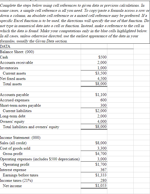
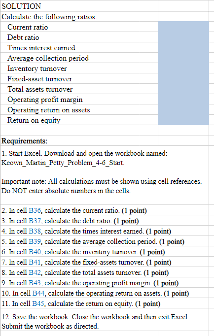
Complete the steps below using cell references to given data or previous calculations. In some cases, a simple cell reference is all you need. To copy paste a formula across a row or down a column, an absolute cell reference or a mixed cell reference may be preferred. If a specific Excel function is to be used, the directions will specify the use of that function. Do not type in numerical data into a cell or function. Instead, make a reference to the cell in which the data is found Make your computations only in the blue cells highlighted below: In all cases, unless otherwise directed, use the earliest appearance of the data in your formulas, usually the Given Data section. DATA Balance Sheet: (000) Cash $500 Accounts receivable 2.000 Inventories 1.000 Current assets $3,500 Net fixed assets 4,500 Total assets $8.000 Accounts payable Accrued expenses Short-term notes payable Current liabilities Long-term debt Owners' equity Total liabilities and owners' equity $1,100 600 300 $2,000 2.000 4.000 $8.000 Income Statement: (000) Sales (all credit) Cost of goods sold Gross profit Operating expenses (includes $500 depreciation) Operating profit Interest expense Earnings before taxes Income taxes (21%) Net income $8.000 3,300 $4,700 3.000 $1,700 367 $1,333 280 $1.053 SOLUTION Calculate the following ratios: Current ratio Debt ratio Times interest earned Average collection period Inventory turnover Fixed-asset turnover Total assets turnover Operating profit margin Operating return on assets Return on equity Requirements: 1. Start Excel. Download and open the workbook named: Keown_Martin_Petty_Problem_4-6_Start. Important note: All calculations must be shown using cell references. Do NOT enter absolute numbers in the cells. 2. In cell B36, calculate the current ratio. (1 point) 3. In cell B37, calculate the debt ratio. (1 point) 4. In cell B38, calculate the times interest earned. (1 point) 5. In cell B39, calculate the average collection period. (1 point) 6. In cell B40, calculate the inventory turnover. (1 point) 7. In cell B41, calculate the fixed-assets turnover. (1 point) 8. In cell B42, calculate the total assets turnover. (1 point) 9. In cell B43, calculate the operating profit margin. (1 point) 10. In cell B44, calculate the operating return on assets. (1 point) 11. In cell B45, calculate the return on equity. (1 point) 12. Save the workbook. Close the workbook and then exit Excel. Submit the workbook as directed