Cost-Volume-Profit Analysis
Using Excel for Cost-Volume-Profit (CVP) Analysis
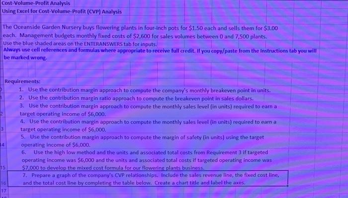
The Oceanside Garden Nursery buys flowering
plants in four-inch pots for $1.50 each and sells
them for $3.00 each. Management budgets
monthly fixed costs of $2,600 for sales volumes
between 0 and 7,500 plants. Use the blue shaded areas on the ENTERANSWERS tab for inputs.
Always use cell references and FORMULAS where
5. Use the contribution margin approach to
compute the margin of safety (in units) using the
target operating income of $6,000.
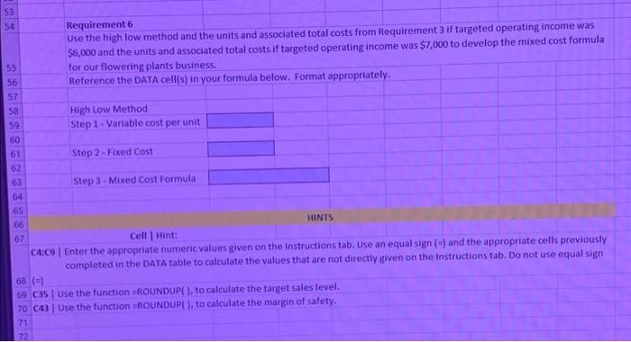
6. Use the high low method and the units and
associated total costs from Requirement 3 if
targeted operating income was $6,000 and the
units and associated total costs if targeted
operating income was $7,000 to develop the
mixed cost formula for our flowering plants
business.
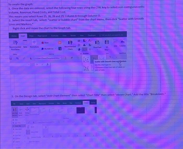
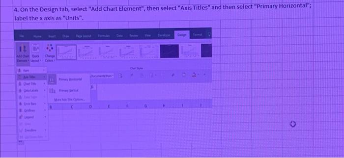
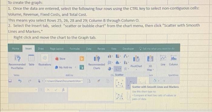
7. Prepare a graph of the company's CVP
relationships. Include the sales revenue line, the
fixed cost line, and the total cost line by
completing the table below. Create a chart title and label the axes. Show the formulas as well please :)
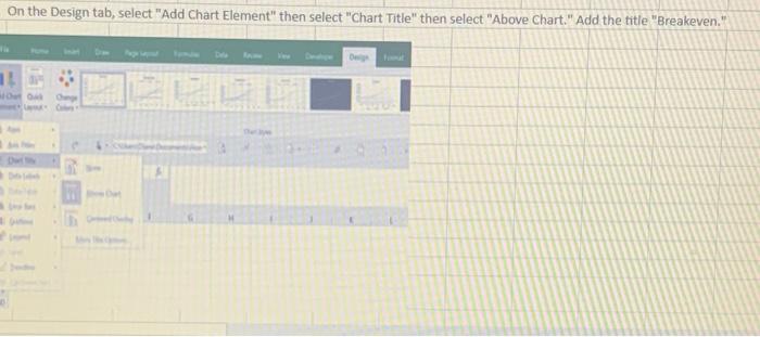
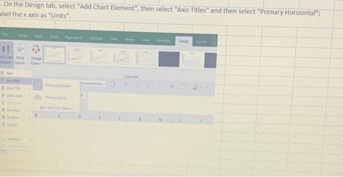
Cost-Volume-Profit Analysis Using Excel for Cost-Volume-Profit (CVP) Analysis The Oceanside Garden Nursery buys flowering plants in four-inch pots for $1.50 each and sells them for $3.00 each Management budgets monthly fixed costs of $2,600 for sales volumes between 0 and 7,500 plants. Use the blue shaded areas on the ENTERANSWERS tab for inputs. Always use cell references and formulas where appropriate to receive full credit. If you copy/paste from the Instructions tab you will be marked wrong. 3 Requirements: 1. Use the contribution margin approach to compute the company's monthly breakeven point in units. 2. Use the contribution margin ratio approach to compute the breakeven point in sales dollars. 3. Use the contribution margin approach to compute the monthly sales level (in units) required to earn a target operating income of $6,000. 4. Use the contribution margin approach to compute the monthly sales level (in units) required to earn a target operating income of $6,000. 5. Use the contribution margin approach to compute the margin of safety (in units) using the target operating income of $6,000. 6. Use the high low method and the units and associated total costs from Requirement 3 if targeted operating income was $6,000 and the units and associated total costs if targeted operating income was 15 $7,000 to develop the mixed cost formula for our flowering plants business. 7. Prepare a graph of the company's CVP relationships. Include the sales revenue line, the fixed cost line, 16 and the total cost line by completing the table below. Create a chart title and label the axes. 17 4 Requirement 5 Use the contribution margin approach to compute the margin of safety (in units) using the target operating income of $6,000. Reference the DATA cell(s) in your formula below. Format as number. Use the Excel ROUNDUP function to obtain whole units to reach the margin of safety Margin of Safety (in units) 53 54 Requirement 6 Use the high low method and the units and associated total costs from Requirement 3 if targeted operating income was $6,000 and the units and associated total costs if targeted operating income was $7,000 to develop the mixed cost formula for our flowering plants business. Reference the DATA cell(s) in your formula below. Format appropriately. 55 56 57 58 59 60 61 High Low Method Step 1. Variable cost per unit Step 2 - Fixed Cost 63 Step 3 - Mixed Cost Formula 64 65 66 HINTS 67 Cell Hint: 04:09 Enter the appropriate numeric values given on the instructions tab. Use an equal sign (=) and the appropriate cells previously completed in the DATA table to calculate the values that are not directly given on the instructions tab. Do not use equal sign 68 (-) 69 C35 Use the function =ROUNDUP(), to calculate the target sales level. 70 C43 Use the function =ROUNDUP(), to calculate the margin of safety. 71 72 5 Chartassistance Create a table to compute the revenue, Variable costs, fixed costs, and total costs for each volume to use in creating your granti DO 0 2.000 400 1,000 200 1.800 2.700 1.400 600 1,600 2.400 07 20 29 30 31 12 33 34 Volume Hever Variable costs Fred Cott Total Cost To create the graph: 1. Once the data are entered, select the following four rows using the CTRL key to select non-contiguous cells: Volume, Revenue, Fixed Costs, and Total Cost. This means you select Rows 25, 26, 28 and 29; Column B through Column O. 2. Select the Insert tab, select "scatter or bubble chart" from the chart menu, then click "Scatter with Smooth Lines and Markers." Right click and move the chart to the Graph tab. Des Pogba Developm Store Recomandat . the color Add Recommended Chat 30 MAD O Seth Cours Scatter with other Use this chat ut du 3. On the Design tab, select "Add Chart Element then select "Chart Title" then select "Above Chart." Add the title "Breakeven." 11 D 4. On the Design tab, select "Add Chart Element", then select "Axis Titles" and then select "Primary Horizontal"; label the xaxis as "Units". Sce 11 MODA D th + To create the graph: 1. Once the data are entered, select the following four rows using the CTRL key to select non-contiguous cells: Volume, Revenue, Fixed Costs, and Total Cost. This means you select Rows 25, 26, 28 and 29; Column B through Column 0. 2. Select the Insert tab, select "scatter or bubble chart" from the chart menu, then click "Scatter with Smooth Lines and Markers." Right click and move the chart to the Graph tab. I Page Layout foman Data Do Tell me what you want to do 1. L. 15 Recommended Phot MA See Che Scatter Under On the Design tab, select "Add Chart Element" then select "Chart Title" then select "Above Chart." Add the title "Breakeven." 11 . On the Design tab, select "Add Chart Element", then select "Axis Titles" and then select "Primary Horizontal"; abel the x axis as "Units". 11 Cost-Volume-Profit Analysis Using Excel for Cost-Volume-Profit (CVP) Analysis The Oceanside Garden Nursery buys flowering plants in four-inch pots for $1.50 each and sells them for $3.00 each Management budgets monthly fixed costs of $2,600 for sales volumes between 0 and 7,500 plants. Use the blue shaded areas on the ENTERANSWERS tab for inputs. Always use cell references and formulas where appropriate to receive full credit. If you copy/paste from the Instructions tab you will be marked wrong. 3 Requirements: 1. Use the contribution margin approach to compute the company's monthly breakeven point in units. 2. Use the contribution margin ratio approach to compute the breakeven point in sales dollars. 3. Use the contribution margin approach to compute the monthly sales level (in units) required to earn a target operating income of $6,000. 4. Use the contribution margin approach to compute the monthly sales level (in units) required to earn a target operating income of $6,000. 5. Use the contribution margin approach to compute the margin of safety (in units) using the target operating income of $6,000. 6. Use the high low method and the units and associated total costs from Requirement 3 if targeted operating income was $6,000 and the units and associated total costs if targeted operating income was 15 $7,000 to develop the mixed cost formula for our flowering plants business. 7. Prepare a graph of the company's CVP relationships. Include the sales revenue line, the fixed cost line, 16 and the total cost line by completing the table below. Create a chart title and label the axes. 17 4 Requirement 5 Use the contribution margin approach to compute the margin of safety (in units) using the target operating income of $6,000. Reference the DATA cell(s) in your formula below. Format as number. Use the Excel ROUNDUP function to obtain whole units to reach the margin of safety Margin of Safety (in units) 53 54 Requirement 6 Use the high low method and the units and associated total costs from Requirement 3 if targeted operating income was $6,000 and the units and associated total costs if targeted operating income was $7,000 to develop the mixed cost formula for our flowering plants business. Reference the DATA cell(s) in your formula below. Format appropriately. 55 56 57 58 59 60 61 High Low Method Step 1. Variable cost per unit Step 2 - Fixed Cost 63 Step 3 - Mixed Cost Formula 64 65 66 HINTS 67 Cell Hint: 04:09 Enter the appropriate numeric values given on the instructions tab. Use an equal sign (=) and the appropriate cells previously completed in the DATA table to calculate the values that are not directly given on the instructions tab. Do not use equal sign 68 (-) 69 C35 Use the function =ROUNDUP(), to calculate the target sales level. 70 C43 Use the function =ROUNDUP(), to calculate the margin of safety. 71 72 5 Chartassistance Create a table to compute the revenue, Variable costs, fixed costs, and total costs for each volume to use in creating your granti DO 0 2.000 400 1,000 200 1.800 2.700 1.400 600 1,600 2.400 07 20 29 30 31 12 33 34 Volume Hever Variable costs Fred Cott Total Cost


