Could you give me a step by step solution on excel for it please!! It'll be a great help for my coming exams !!! will thumbs up

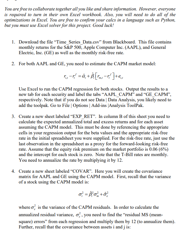
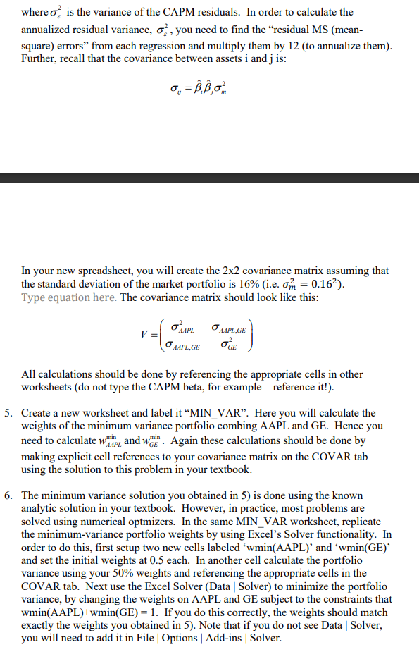
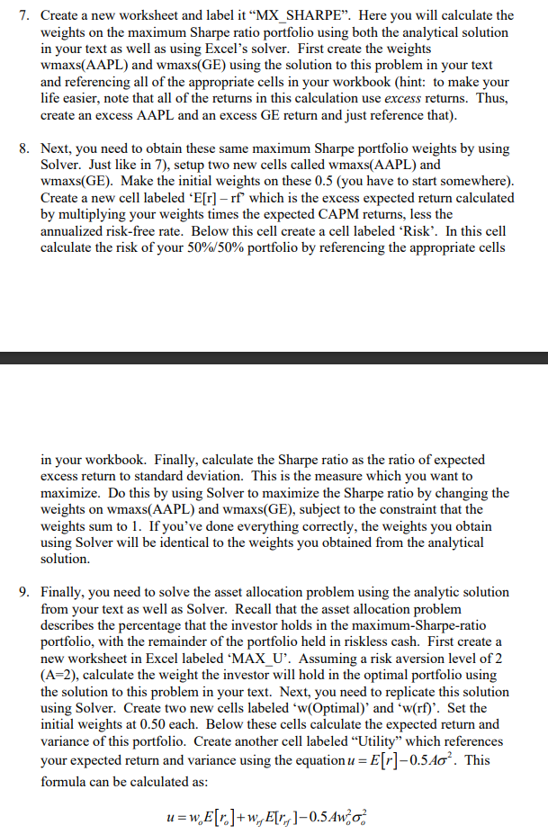
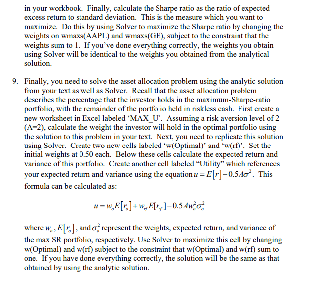
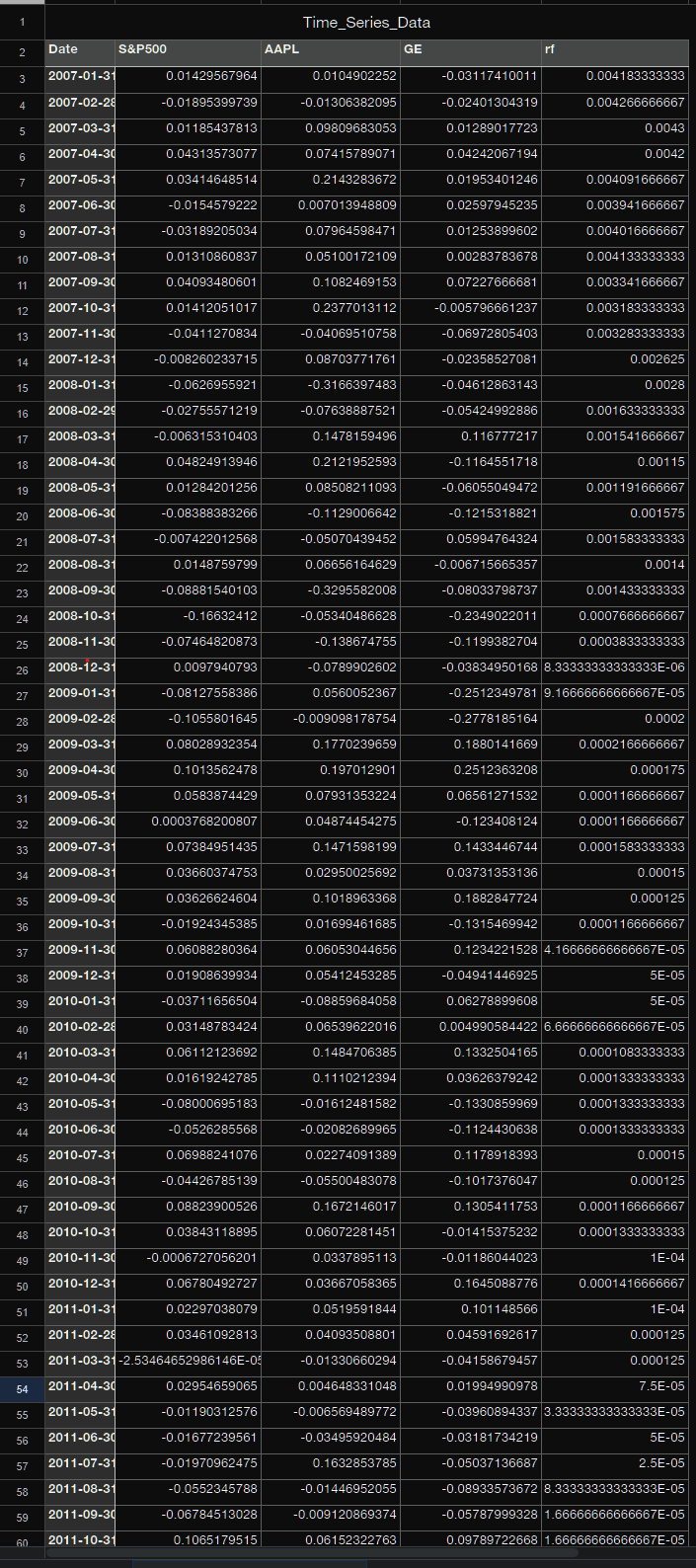
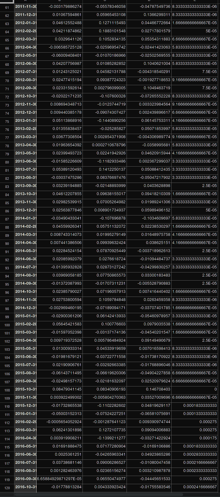
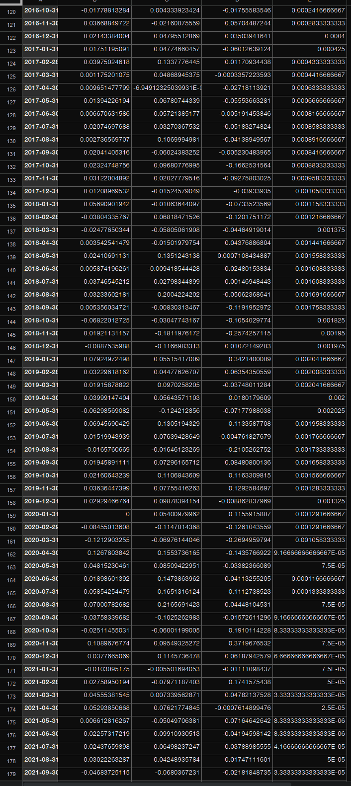
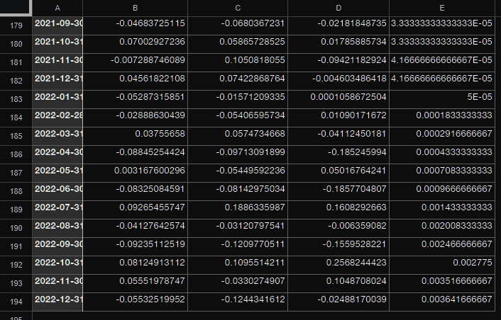
You are free to collaborate together all you like and share information. However, everyone is required to turn in their own Excel workbook. Also, you will need to do all of the optimizations in Excel. You are free to confirm your calcs in a language such as Python, but you must use Excel solver for this project. Good luck! 1. Download the file "Time_Series_Data.csv" from Blackboard. This file contains monthly returns for the S\& 500 , Apple Computer Inc. (AAPL), and General Electric, Inc. (GE) as well as the monthly risk-free rate. 2. For both AAPL and GE, you need to estimate the CAPM market model: ri,trtf=^i+^i[rm,trtf]+ei,t Use Excel to run the CAPM regression for both stocks. Output the results to a new tab for each security and label the tabs "AAPL_CAPM" and "GE_CAPM", respectively. Note that if you do not see Data | Data Analysis, you likely need to add the toolpak. Go to File | Options | Add-ins |Analysis ToolPak. 3. Create a new sheet labeled "EXP_RET". In column B of this sheet you need to calculate the expected annualized total and excess returns and for each asset assuming the CAPM model. This must be done by referencing the appropriate cells in your regression output for the beta values and the appropriate risk-free rate in the initial spreadsheet you were supplied. For the risk-free rate, just use the last observation in the spreadsheet as a proxy for the forward-looking risk-free rate. Assume that the equity risk premium on the market portfolio is 0.06(6%) and the intercept for each stock is zero. Note that the T-Bill rates are monthly. You need to annualize the rate by multiplying it by 12 . 4. Create a new sheet labeled "COVAR". Here you will create the covariance matrix for AAPL and GE using the CAPM model. First, recall that the variance of a stock using the CAPM model is: i2=^i2m2+^2 where 2 is the variance of the CAPM residuals. In order to calculate the annualized residual variance, e2, you need to find the "residual MS (meansquare) errors" from each regression and multiply them by 12 (to annualize them). Further, recall that the covariance between assets i and j is: where 2 is the variance of the CAPM residuals. In order to calculate the annualized residual variance, 2, you need to find the "residual MS (meansquare) errors" from each regression and multiply them by 12 (to annualize them). Further, recall that the covariance between assets i and j is: ij=^i^jm2 In your new spreadsheet, you will create the 22 covariance matrix assuming that the standard deviation of the market portfolio is 16% (i.e. m2=0.162 ). Type equation here. The covariance matrix should look like this: V=(AAPL2AAPL,GEAAPL,GEGE2) All calculations should be done by referencing the appropriate cells in other worksheets (do not type the CAPM beta, for example - reference it!). 5. Create a new worksheet and label it "MIN_VAR". Here you will calculate the weights of the minimum variance portfolio combing AAPL and GE. Hence you need to calculate wAAPLmin and wGEmin. Again these calculations should be done by making explicit cell references to your covariance matrix on the COVAR tab using the solution to this problem in your textbook. 6. The minimum variance solution you obtained in 5) is done using the known analytic solution in your textbook. However, in practice, most problems are solved using numerical optmizers. In the same MIN_VAR worksheet, replicate the minimum-variance portfolio weights by using Excel's Solver functionality. In order to do this, first setup two new cells labeled 'wmin(AAPL)' and 'wmin(GE)' and set the initial weights at 0.5 each. In another cell calculate the portfolio variance using your 50% weights and referencing the appropriate cells in the COVAR tab. Next use the Excel Solver (Data | Solver) to minimize the portfolio variance, by changing the weights on AAPL and GE subject to the constraints that wmin(AAPL)+wmin(GE) = 1. If you do this correctly, the weights should match exactly the weights you obtained in 5). Note that if you do not see Data | Solver, you will need to add it in File Options Add-ins Solver. 7. Create a new worksheet and label it "MX_SHARPE". Here you will calculate the weights on the maximum Sharpe ratio portfolio using both the analytical solution in your text as well as using Excel's solver. First create the weights wmaxs(AAPL) and wmaxs(GE) using the solution to this problem in your text and referencing all of the appropriate cells in your workbook (hint: to make your life easier, note that all of the returns in this calculation use excess returns. Thus, create an excess AAPL and an excess GE return and just reference that). 8. Next, you need to obtain these same maximum Sharpe portfolio weights by using Solver. Just like in 7), setup two new cells called wmaxs(AAPL) and wmaxs(GE). Make the initial weights on these 0.5 (you have to start somewhere). Create a new cell labeled ' E[r] - rf ' which is the excess expected return calculated by multiplying your weights times the expected CAPM returns, less the annualized risk-free rate. Below this cell create a cell labeled 'Risk'. In this cell calculate the risk of your 50%/50% portfolio by referencing the appropriate cells in your workbook. Finally, calculate the Sharpe ratio as the ratio of expected excess return to standard deviation. This is the measure which you want to maximize. Do this by using Solver to maximize the Sharpe ratio by changing the weights on wmaxs(AAPL) and wmaxs(GE), subject to the constraint that the weights sum to 1 . If you've done everything correctly, the weights you obtain using Solver will be identical to the weights you obtained from the analytical solution. 9. Finally, you need to solve the asset allocation problem using the analytic solution from your text as well as Solver. Recall that the asset allocation problem describes the percentage that the investor holds in the maximum-Sharpe-ratio portfolio, with the remainder of the portfolio held in riskless cash. First create a new worksheet in Excel labeled 'MAX_U'. Assuming a risk aversion level of 2 (A=2), calculate the weight the investor will hold in the optimal portfolio using the solution to this problem in your text. Next, you need to replicate this solution using Solver. Create two new cells labeled 'w(Optimal)' and 'w(rf)'. Set the initial weights at 0.50 each. Below these cells calculate the expected return and variance of this portfolio. Create another cell labeled "Utility" which references your expected return and variance using the equation u=E[r]0.5A2. This formula can be calculated as: u=woE[ro]+wrfE[rrf]0.5Awo2o2 in your workbook. Finally, calculate the Sharpe ratio as the ratio of expected excess return to standard deviation. This is the measure which you want to maximize. Do this by using Solver to maximize the Sharpe ratio by changing the weights on wmaxs(AAPL) and wmaxs(GE), subject to the constraint that the weights sum to 1 . If you've done everything correctly, the weights you obtain using Solver will be identical to the weights you obtained from the analytical solution. Finally, you need to solve the asset allocation problem using the analytic solution from your text as well as Solver. Recall that the asset allocation problem describes the percentage that the investor holds in the maximum-Sharpe-ratio portfolio, with the remainder of the portfolio held in riskless cash. First create a new worksheet in Excel labeled 'MAX_U'. Assuming a risk aversion level of 2 (A=2), calculate the weight the investor will hold in the optimal portfolio using the solution to this problem in your text. Next, you need to replicate this solution using Solver. Create two new cells labeled 'w(Optimal)' and 'w(rf)'. Set the initial weights at 0.50 each. Below these cells calculate the expected return and variance of this portfolio. Create another cell labeled "Utility" which references your expected return and variance using the equation u=E[r]0.5A2. This formula can be calculated as: u=woE[ro]+wrfE[rrf]0.5Awo2o2 where wo,E[ro], and o2 represent the weights, expected return, and variance of the max SR portfolio, respectively. Use Solver to maximize this cell by changing w( Optimal) and w(rf) subject to the constraint that w(Optimal) and w(rf) sum to one. If you have done everything correctly, the solution will be the same as that obtained by using the analytic solution. You are free to collaborate together all you like and share information. However, everyone is required to turn in their own Excel workbook. Also, you will need to do all of the optimizations in Excel. You are free to confirm your calcs in a language such as Python, but you must use Excel solver for this project. Good luck! 1. Download the file "Time_Series_Data.csv" from Blackboard. This file contains monthly returns for the S\& 500 , Apple Computer Inc. (AAPL), and General Electric, Inc. (GE) as well as the monthly risk-free rate. 2. For both AAPL and GE, you need to estimate the CAPM market model: ri,trtf=^i+^i[rm,trtf]+ei,t Use Excel to run the CAPM regression for both stocks. Output the results to a new tab for each security and label the tabs "AAPL_CAPM" and "GE_CAPM", respectively. Note that if you do not see Data | Data Analysis, you likely need to add the toolpak. Go to File | Options | Add-ins |Analysis ToolPak. 3. Create a new sheet labeled "EXP_RET". In column B of this sheet you need to calculate the expected annualized total and excess returns and for each asset assuming the CAPM model. This must be done by referencing the appropriate cells in your regression output for the beta values and the appropriate risk-free rate in the initial spreadsheet you were supplied. For the risk-free rate, just use the last observation in the spreadsheet as a proxy for the forward-looking risk-free rate. Assume that the equity risk premium on the market portfolio is 0.06(6%) and the intercept for each stock is zero. Note that the T-Bill rates are monthly. You need to annualize the rate by multiplying it by 12 . 4. Create a new sheet labeled "COVAR". Here you will create the covariance matrix for AAPL and GE using the CAPM model. First, recall that the variance of a stock using the CAPM model is: i2=^i2m2+^2 where 2 is the variance of the CAPM residuals. In order to calculate the annualized residual variance, e2, you need to find the "residual MS (meansquare) errors" from each regression and multiply them by 12 (to annualize them). Further, recall that the covariance between assets i and j is: where 2 is the variance of the CAPM residuals. In order to calculate the annualized residual variance, 2, you need to find the "residual MS (meansquare) errors" from each regression and multiply them by 12 (to annualize them). Further, recall that the covariance between assets i and j is: ij=^i^jm2 In your new spreadsheet, you will create the 22 covariance matrix assuming that the standard deviation of the market portfolio is 16% (i.e. m2=0.162 ). Type equation here. The covariance matrix should look like this: V=(AAPL2AAPL,GEAAPL,GEGE2) All calculations should be done by referencing the appropriate cells in other worksheets (do not type the CAPM beta, for example - reference it!). 5. Create a new worksheet and label it "MIN_VAR". Here you will calculate the weights of the minimum variance portfolio combing AAPL and GE. Hence you need to calculate wAAPLmin and wGEmin. Again these calculations should be done by making explicit cell references to your covariance matrix on the COVAR tab using the solution to this problem in your textbook. 6. The minimum variance solution you obtained in 5) is done using the known analytic solution in your textbook. However, in practice, most problems are solved using numerical optmizers. In the same MIN_VAR worksheet, replicate the minimum-variance portfolio weights by using Excel's Solver functionality. In order to do this, first setup two new cells labeled 'wmin(AAPL)' and 'wmin(GE)' and set the initial weights at 0.5 each. In another cell calculate the portfolio variance using your 50% weights and referencing the appropriate cells in the COVAR tab. Next use the Excel Solver (Data | Solver) to minimize the portfolio variance, by changing the weights on AAPL and GE subject to the constraints that wmin(AAPL)+wmin(GE) = 1. If you do this correctly, the weights should match exactly the weights you obtained in 5). Note that if you do not see Data | Solver, you will need to add it in File Options Add-ins Solver. 7. Create a new worksheet and label it "MX_SHARPE". Here you will calculate the weights on the maximum Sharpe ratio portfolio using both the analytical solution in your text as well as using Excel's solver. First create the weights wmaxs(AAPL) and wmaxs(GE) using the solution to this problem in your text and referencing all of the appropriate cells in your workbook (hint: to make your life easier, note that all of the returns in this calculation use excess returns. Thus, create an excess AAPL and an excess GE return and just reference that). 8. Next, you need to obtain these same maximum Sharpe portfolio weights by using Solver. Just like in 7), setup two new cells called wmaxs(AAPL) and wmaxs(GE). Make the initial weights on these 0.5 (you have to start somewhere). Create a new cell labeled ' E[r] - rf ' which is the excess expected return calculated by multiplying your weights times the expected CAPM returns, less the annualized risk-free rate. Below this cell create a cell labeled 'Risk'. In this cell calculate the risk of your 50%/50% portfolio by referencing the appropriate cells in your workbook. Finally, calculate the Sharpe ratio as the ratio of expected excess return to standard deviation. This is the measure which you want to maximize. Do this by using Solver to maximize the Sharpe ratio by changing the weights on wmaxs(AAPL) and wmaxs(GE), subject to the constraint that the weights sum to 1 . If you've done everything correctly, the weights you obtain using Solver will be identical to the weights you obtained from the analytical solution. 9. Finally, you need to solve the asset allocation problem using the analytic solution from your text as well as Solver. Recall that the asset allocation problem describes the percentage that the investor holds in the maximum-Sharpe-ratio portfolio, with the remainder of the portfolio held in riskless cash. First create a new worksheet in Excel labeled 'MAX_U'. Assuming a risk aversion level of 2 (A=2), calculate the weight the investor will hold in the optimal portfolio using the solution to this problem in your text. Next, you need to replicate this solution using Solver. Create two new cells labeled 'w(Optimal)' and 'w(rf)'. Set the initial weights at 0.50 each. Below these cells calculate the expected return and variance of this portfolio. Create another cell labeled "Utility" which references your expected return and variance using the equation u=E[r]0.5A2. This formula can be calculated as: u=woE[ro]+wrfE[rrf]0.5Awo2o2 in your workbook. Finally, calculate the Sharpe ratio as the ratio of expected excess return to standard deviation. This is the measure which you want to maximize. Do this by using Solver to maximize the Sharpe ratio by changing the weights on wmaxs(AAPL) and wmaxs(GE), subject to the constraint that the weights sum to 1 . If you've done everything correctly, the weights you obtain using Solver will be identical to the weights you obtained from the analytical solution. Finally, you need to solve the asset allocation problem using the analytic solution from your text as well as Solver. Recall that the asset allocation problem describes the percentage that the investor holds in the maximum-Sharpe-ratio portfolio, with the remainder of the portfolio held in riskless cash. First create a new worksheet in Excel labeled 'MAX_U'. Assuming a risk aversion level of 2 (A=2), calculate the weight the investor will hold in the optimal portfolio using the solution to this problem in your text. Next, you need to replicate this solution using Solver. Create two new cells labeled 'w(Optimal)' and 'w(rf)'. Set the initial weights at 0.50 each. Below these cells calculate the expected return and variance of this portfolio. Create another cell labeled "Utility" which references your expected return and variance using the equation u=E[r]0.5A2. This formula can be calculated as: u=woE[ro]+wrfE[rrf]0.5Awo2o2 where wo,E[ro], and o2 represent the weights, expected return, and variance of the max SR portfolio, respectively. Use Solver to maximize this cell by changing w( Optimal) and w(rf) subject to the constraint that w(Optimal) and w(rf) sum to one. If you have done everything correctly, the solution will be the same as that obtained by using the analytic solution