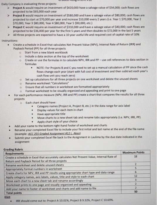
CREATE A SCHEDULE IN EXCEL THAT CALCULATES NPV, IRR, and PP for all three projects.

Daily Company is evaluating three projects Project A would require an investment of $420,000 have a salvage value of $54,000; cash flows are projected to be $65,000 each year Project B would require an investment of $580,000 and have a salvage value of $80,000; cash flows are projected to start at $70,000 per year and increase $10,000 every 2 years (i.e. Year 1 $70,000, Year 2 $70,000, Year 3 $80,000, Year 4 $80,000, Year 5 $90,000, etc) Project C would require an investment of $310,000 and have a salvage value of $40,000; cash flows are projected to be $36,000 per year for the first 5 years and then doubles to $72,000 in the last 5 years All three projects are expected to have a 10y > Instructions . Create a schedule in Excel that calculates Net Present Value (NPV), Internal Rate of Return (IRR) and Payback Period (PP) for all three projects o o o Start from a new blank workbook Include a data section at the top of the worksheet Create or use the formulas in to calculate NPV, IRR and PP- use cell references to data section in formulas NOTE: For Projects 8 and C you need to set up a manual calculation of PP since the cash flows change each year (start with full cost of investment and then subtract each years cash flow unit you reach zero) o Set up calculations for alll three projects on one worksheet and delete the unused sheets o Rename worksheet "Calculations Ensure that all numbers in worksheet are formatted appropriately Format worksheet to be visually organized and appealing and print to one page o o For each performance measure (NPV, IRR and PP) create a chart that compares the results for all three projects o Each chart should have: .Category names (Project A, Project 8, etc.) in the data range for axis label Display values for each item in chart .Have appropriate title Move charts to a new sheet tab and rename tabs appropriately (i.e. NPV, IRR, PP) Apply chart style of your choice Add your name to the bottom right-hand footer of worksheet and charts . Rename your completed Excel file to include your first initial and last name at the end of the file name (example: ACC 255 Graded Assignment 812 Ake) Submit your completed Excel file back to the Assignment in Laulima by the due date indicated in the assignment Grading Rubric Maximum Points Requirements Create a schedule in Excel that accurately calculates Net Present Value, Internal Rate of Return and Payback Period for all three projects Rename worksheet and delete unused sheets Appropriately format numbers in worksheet Create charts for NPV, IRR and PP results using appropriate chart type and data range Apply category names, axis labels, values, title and style to each chart Move each chart to a new sheet tab and rename accordingy Worksheet prints to one page and visually organized and appealing Add your name to footer of worksheet and charts and add name to file Total points 18 12 50 Hint IRR should come out to: Project A 10.01%, Project B 9.32%, Project C 10.69%, . Daily Company is evaluating three projects Project A would require an investment of $420,000 have a salvage value of $54,000; cash flows are projected to be $65,000 each year Project B would require an investment of $580,000 and have a salvage value of $80,000; cash flows are projected to start at $70,000 per year and increase $10,000 every 2 years (i.e. Year 1 $70,000, Year 2 $70,000, Year 3 $80,000, Year 4 $80,000, Year 5 $90,000, etc) Project C would require an investment of $310,000 and have a salvage value of $40,000; cash flows are projected to be $36,000 per year for the first 5 years and then doubles to $72,000 in the last 5 years All three projects are expected to have a 10y > Instructions . Create a schedule in Excel that calculates Net Present Value (NPV), Internal Rate of Return (IRR) and Payback Period (PP) for all three projects o o o Start from a new blank workbook Include a data section at the top of the worksheet Create or use the formulas in to calculate NPV, IRR and PP- use cell references to data section in formulas NOTE: For Projects 8 and C you need to set up a manual calculation of PP since the cash flows change each year (start with full cost of investment and then subtract each years cash flow unit you reach zero) o Set up calculations for alll three projects on one worksheet and delete the unused sheets o Rename worksheet "Calculations Ensure that all numbers in worksheet are formatted appropriately Format worksheet to be visually organized and appealing and print to one page o o For each performance measure (NPV, IRR and PP) create a chart that compares the results for all three projects o Each chart should have: .Category names (Project A, Project 8, etc.) in the data range for axis label Display values for each item in chart .Have appropriate title Move charts to a new sheet tab and rename tabs appropriately (i.e. NPV, IRR, PP) Apply chart style of your choice Add your name to the bottom right-hand footer of worksheet and charts . Rename your completed Excel file to include your first initial and last name at the end of the file name (example: ACC 255 Graded Assignment 812 Ake) Submit your completed Excel file back to the Assignment in Laulima by the due date indicated in the assignment Grading Rubric Maximum Points Requirements Create a schedule in Excel that accurately calculates Net Present Value, Internal Rate of Return and Payback Period for all three projects Rename worksheet and delete unused sheets Appropriately format numbers in worksheet Create charts for NPV, IRR and PP results using appropriate chart type and data range Apply category names, axis labels, values, title and style to each chart Move each chart to a new sheet tab and rename accordingy Worksheet prints to one page and visually organized and appealing Add your name to footer of worksheet and charts and add name to file Total points 18 12 50 Hint IRR should come out to: Project A 10.01%, Project B 9.32%, Project C 10.69%


