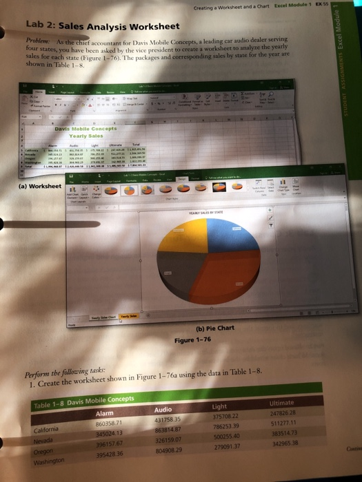
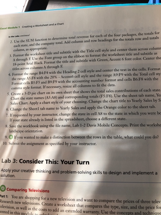
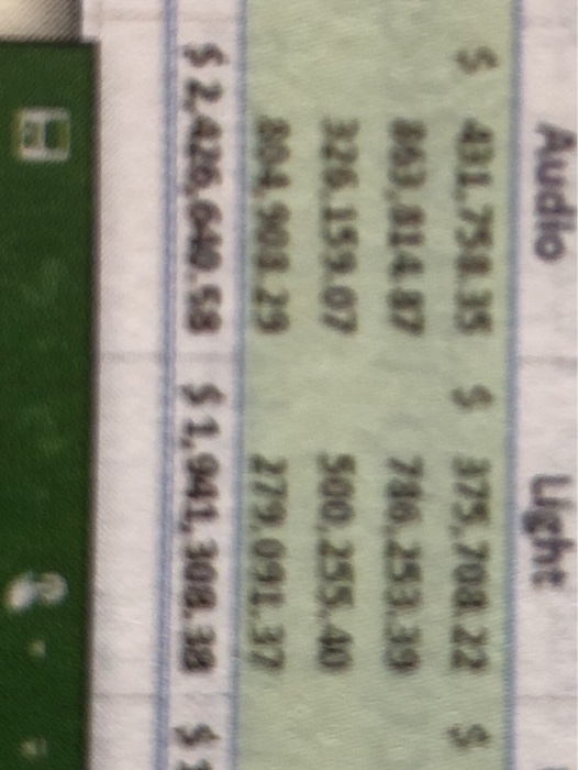
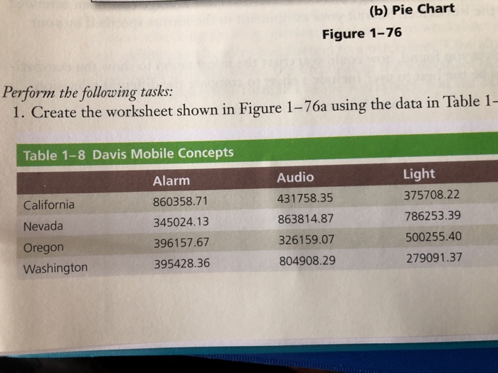
Creating a Worksheet and a Chart Excel Module 1 EX 55 Lab 2: Sales Analysis Worksheet Problem: As the ch W: As the chief accountant for Davis Mobile Concepts, a leading car audio dealer serving Tour states, you have been asked the vice president to create a worksheet to analyze the yearly Sales for each state (Figure 1-76). The packages and corresponding sales by state for the year are shown in Table 1-8 STUDENT ASSIGNMENTS Excel Module 1 De (a) Worksheet (b) Pie Chart Figure 1-76 Perform the following tasks: 1. Create the worksheet shown in Figure 1 - 76a using the data in Table 1-8. Table 1-8 Davis Mobile Concepts Alarm 860358 71 345024.13 39615767 395428 36 Calidornia Nevada Oregon Washington Audio 431758.35 86381487 326159.07 804908 29 Light 375708 22 786253 39 500255.40 27909137 Ultimate 247826 28 511277.11 38351473 34296538 Excel Module 1 Creating a Worksheet and a Chart in the Labacowad 2. Use the SUM function to determine total revenue for each of the four packages, the totals for cach state, and the company total. Add column and row headings for the totals row and totals column, as appropriate. 3. Format the worksheet title and subtitle with the Title cell style and center them across column A through E Use the Font group on the ribbon to format the worksheet title and subtitle as 18-point Arial Black. Format the title and subtitle with Green, Accent 6 font color. Center the titles across columns A through E 4. Format the range B4:F4 with the Heading 2 cell style and center the text in the cells. Format the range A5:F8 with the 20% - Accento cell style and the range A9:F9 with the Total cell sty Format cells B5:55 and B9:F9 with the accounting number format and cells B6:F8 with the comma style format. If necessary, resize all columns to fit the data. 5. Create a 3-D pie chart on its own sheet that shows the total sales contributions of each state. Chart the state names (A5:A8) and corresponding totals (F5:F8). Use the sheet tab name, Ye: Sales Chart. Apply a chart style of your choosing. Change the chart title to Yearly Sales by S 6. Change the Sheetl tab name to Yearly Sales and apply the Orange color to the sheet tab. 7. If requested by your instructor, change the state in cell A8 to the state in which you were bo If your state already is listed in the spreadsheet, choose a different state. 8. Save the workbook using the file name, Lab 1-2 Davis Mobile Concepts. Print the workshe landscape orientation. 9. If you wanted to make a distinction between the rows in the table, what could you do? 10. Submit the assignment as specified by your instructor. Lab 3: Consider This: Your Turn Apply your creative thinking and problem-solving skills to design and implement a solution. Comparing Televisions Part 1: You are shopping for a new television and want to compare the prices of three telev Research new televisions. Create a worksheet that compares the type, size, and the price for celevision, as well as the costs to add an extended warranty. Use the concepts and technique ented in this module to calaulu (b) Pie Chart Figure 1-76 Perform the following tasks: 1. Create the worksheet shown in Figure 1-76a using the data in Table 1- Table 1-8 Davis Mobile Concepts California Nevada Oregon Washington Alarm 860358.71 345024.13 396157.67 395428.36 Audio 431758.35 863814.87 326159.07 804908.29 Light 375708.22 786253.39 500255.40 279091.37 Creating a Worksheet and a Chart Excel Module 1 EX 55 Lab 2: Sales Analysis Worksheet Problem: As the ch W: As the chief accountant for Davis Mobile Concepts, a leading car audio dealer serving Tour states, you have been asked the vice president to create a worksheet to analyze the yearly Sales for each state (Figure 1-76). The packages and corresponding sales by state for the year are shown in Table 1-8 STUDENT ASSIGNMENTS Excel Module 1 De (a) Worksheet (b) Pie Chart Figure 1-76 Perform the following tasks: 1. Create the worksheet shown in Figure 1 - 76a using the data in Table 1-8. Table 1-8 Davis Mobile Concepts Alarm 860358 71 345024.13 39615767 395428 36 Calidornia Nevada Oregon Washington Audio 431758.35 86381487 326159.07 804908 29 Light 375708 22 786253 39 500255.40 27909137 Ultimate 247826 28 511277.11 38351473 34296538 Excel Module 1 Creating a Worksheet and a Chart in the Labacowad 2. Use the SUM function to determine total revenue for each of the four packages, the totals for cach state, and the company total. Add column and row headings for the totals row and totals column, as appropriate. 3. Format the worksheet title and subtitle with the Title cell style and center them across column A through E Use the Font group on the ribbon to format the worksheet title and subtitle as 18-point Arial Black. Format the title and subtitle with Green, Accent 6 font color. Center the titles across columns A through E 4. Format the range B4:F4 with the Heading 2 cell style and center the text in the cells. Format the range A5:F8 with the 20% - Accento cell style and the range A9:F9 with the Total cell sty Format cells B5:55 and B9:F9 with the accounting number format and cells B6:F8 with the comma style format. If necessary, resize all columns to fit the data. 5. Create a 3-D pie chart on its own sheet that shows the total sales contributions of each state. Chart the state names (A5:A8) and corresponding totals (F5:F8). Use the sheet tab name, Ye: Sales Chart. Apply a chart style of your choosing. Change the chart title to Yearly Sales by S 6. Change the Sheetl tab name to Yearly Sales and apply the Orange color to the sheet tab. 7. If requested by your instructor, change the state in cell A8 to the state in which you were bo If your state already is listed in the spreadsheet, choose a different state. 8. Save the workbook using the file name, Lab 1-2 Davis Mobile Concepts. Print the workshe landscape orientation. 9. If you wanted to make a distinction between the rows in the table, what could you do? 10. Submit the assignment as specified by your instructor. Lab 3: Consider This: Your Turn Apply your creative thinking and problem-solving skills to design and implement a solution. Comparing Televisions Part 1: You are shopping for a new television and want to compare the prices of three telev Research new televisions. Create a worksheet that compares the type, size, and the price for celevision, as well as the costs to add an extended warranty. Use the concepts and technique ented in this module to calaulu (b) Pie Chart Figure 1-76 Perform the following tasks: 1. Create the worksheet shown in Figure 1-76a using the data in Table 1- Table 1-8 Davis Mobile Concepts California Nevada Oregon Washington Alarm 860358.71 345024.13 396157.67 395428.36 Audio 431758.35 863814.87 326159.07 804908.29 Light 375708.22 786253.39 500255.40 279091.37