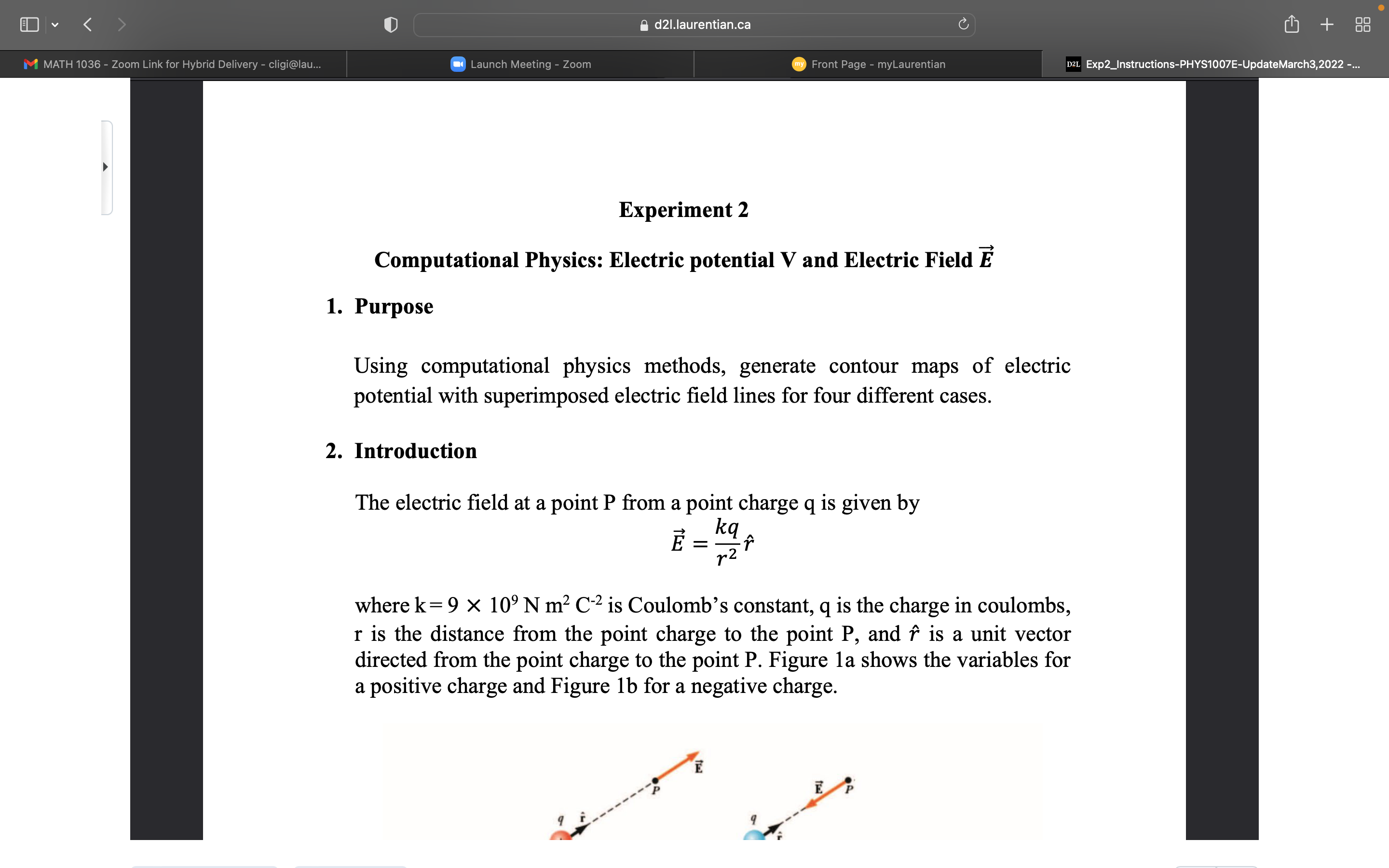
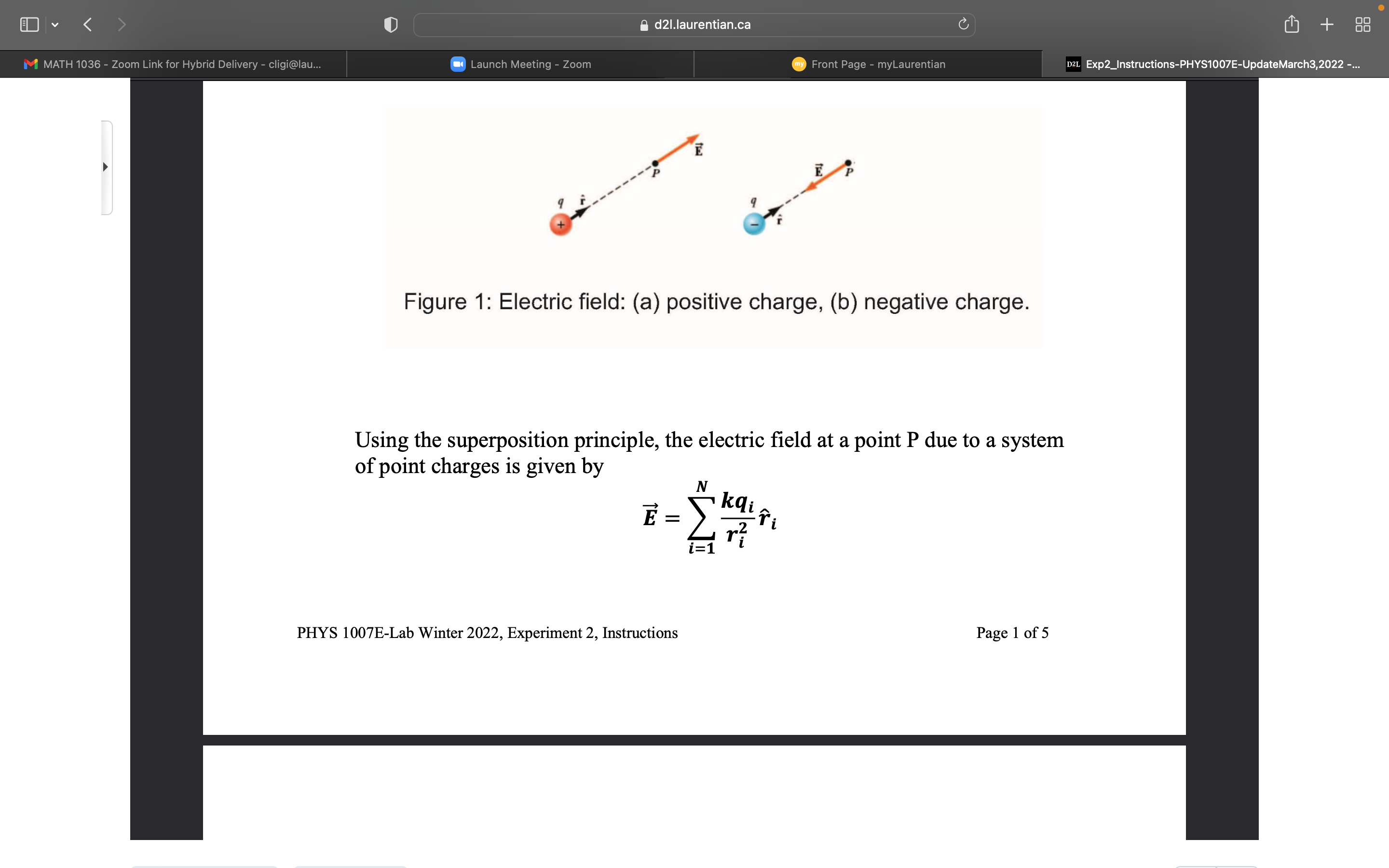
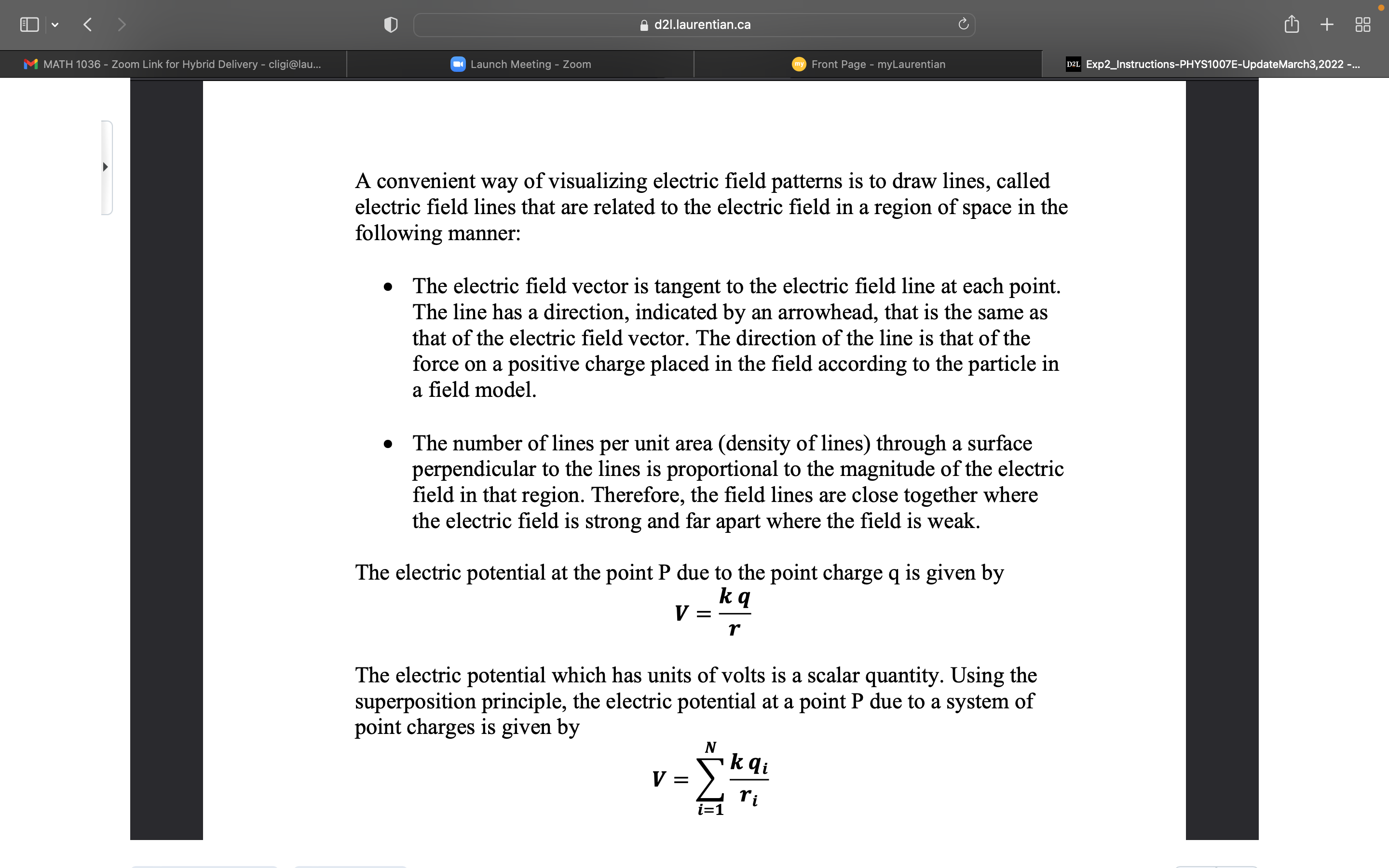
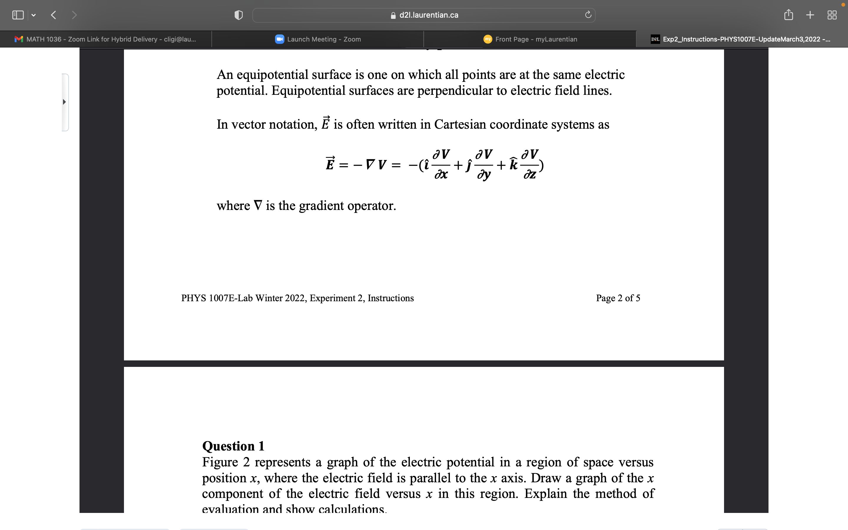
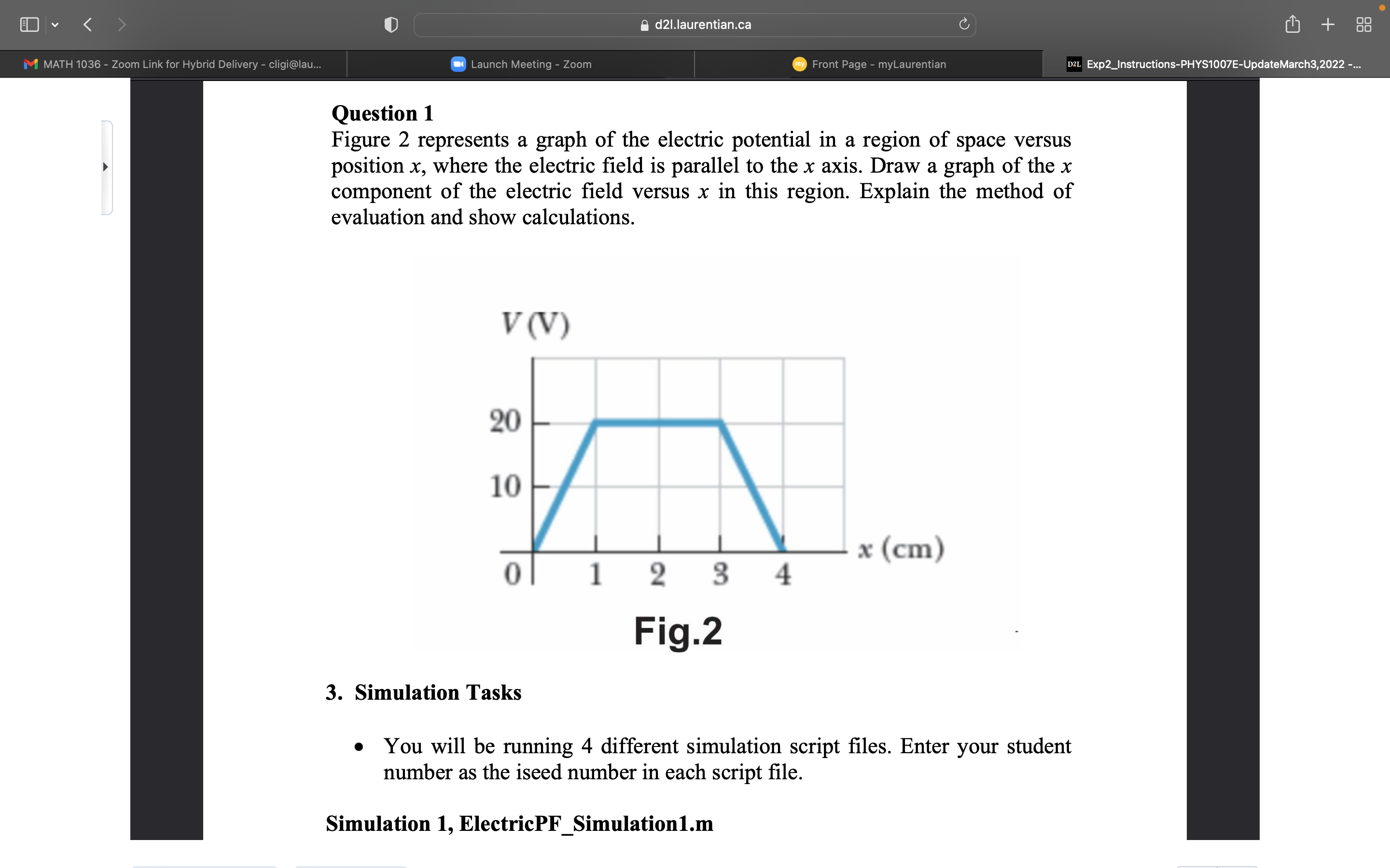
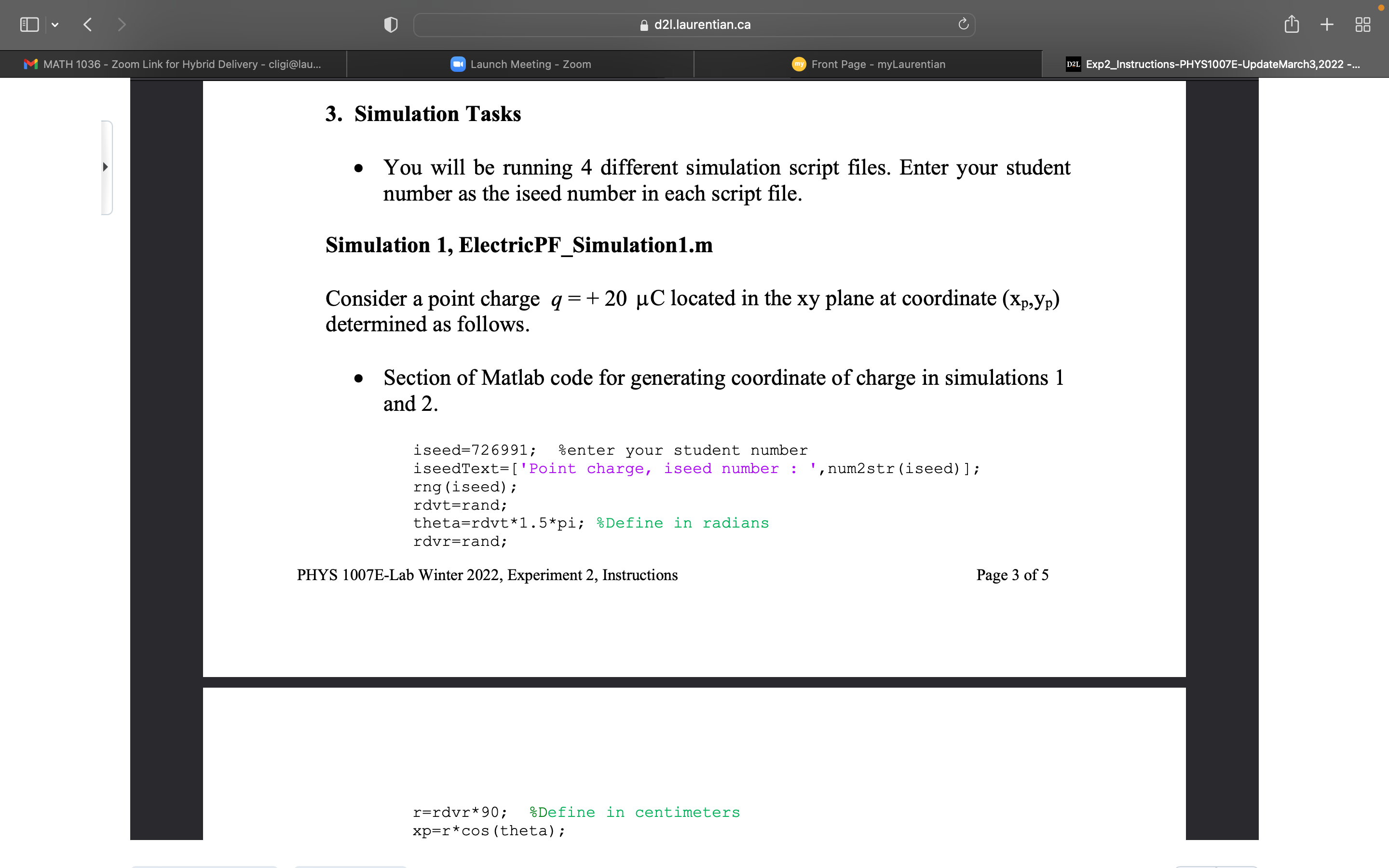
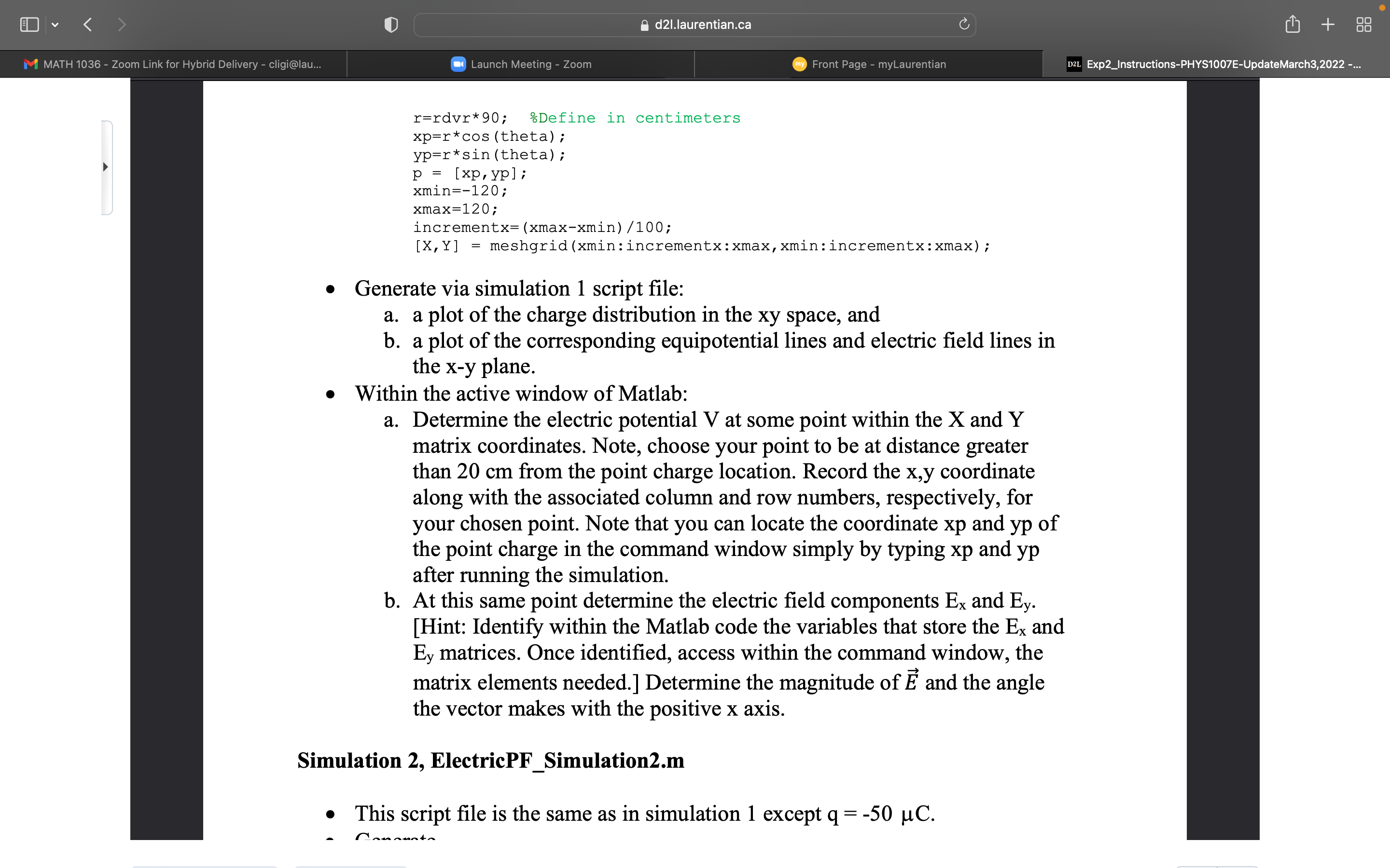
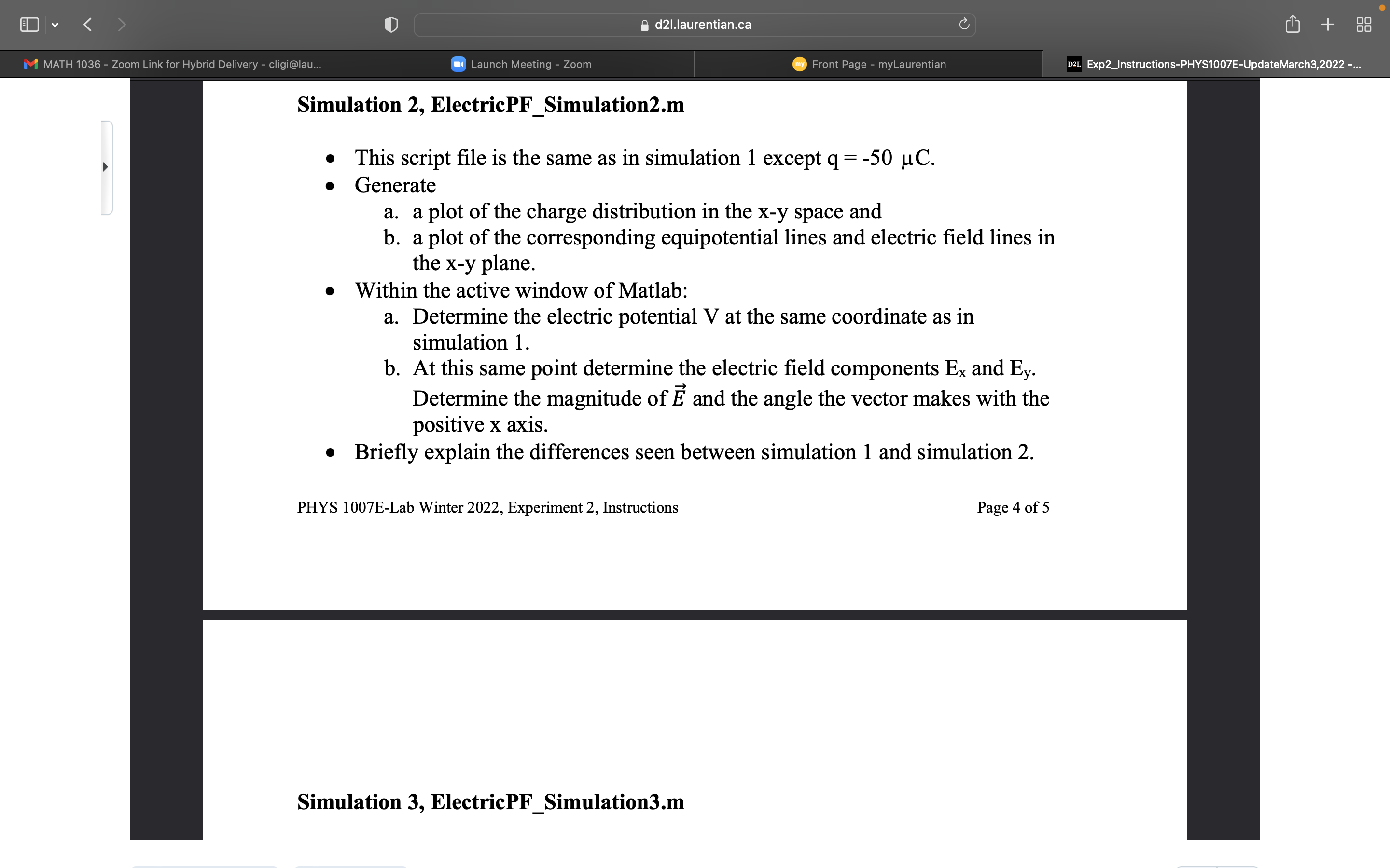
d21.laurentian.ca C + M MATH 1036 - Zoom Link for Hybrid Delivery - cligi@lau... Launch Meeting - Zoom my Front Page - myLaurentian D2L Exp2_Instructions-PHYS1007E-UpdateMarch3,2022 -... Experiment 2 Computational Physics: Electric potential V and Electric Field E 1. Purpose Using computational physics methods, generate contour maps of electric potential with superimposed electric field lines for four different cases. 2. Introduction The electric field at a point P from a point charge q is given by E = kq where k = 9 X 109 N m2 C-2 is Coulomb's constant, q is the charge in coulombs, r is the distance from the point charge to the point P, and f is a unit vector directed from the point charge to the point P. Figure la shows the variables for a positive charge and Figure 1b for a negative charge. Ed21.laurentian.ca C + M MATH 1036 - Zoom Link for Hybrid Delivery - cligi@lau... Launch Meeting - Zoom my Front Page - myLaurentian D2L Exp2_Instructions-PHYS1007E-UpdateMarch3,2022 -... E Figure 1: Electric field: (a) positive charge, (b) negative charge. Using the superposition principle, the electric field at a point P due to a system of point charges is given by E = kairi i=1 PHYS 1007E-Lab Winter 2022, Experiment 2, Instructions Page 1 of 5d21.laurentian.ca C + M MATH 1036 - Zoom Link for Hybrid Delivery - cligi@lau... Launch Meeting - Zoom my Front Page - myLaurentian D2L Exp2_Instructions-PHYS1007E-UpdateMarch3,2022 -... A convenient way of visualizing electric field patterns is to draw lines, called electric field lines that are related to the electric field in a region of space in the following manner: . The electric field vector is tangent to the electric field line at each point. The line has a direction, indicated by an arrowhead, that is the same as that of the electric field vector. The direction of the line is that of the force on a positive charge placed in the field according to the particle in a field model. . The number of lines per unit area (density of lines) through a surface perpendicular to the lines is proportional to the magnitude of the electric field in that region. Therefore, the field lines are close together where the electric field is strong and far apart where the field is weak. The electric potential at the point P due to the point charge q is given by V = kq The electric potential which has units of volts is a scalar quantity. Using the superposition principle, the electric potential at a point P due to a system of point charges is given by 12 V = k qi ri i=1d2l.laurentian.ca C + M MATH 1036 - Zoom Link for Hybrid Delivery - cligi@lau... Launch Meeting - Zoom my Front Page - myLaurentian D2L Exp2_Instructions-PHYS1007E-UpdateMarch3,2022 -... An equipotential surface is one on which all points are at the same electric potential. Equipotential surfaces are perpendicular to electric field lines. In vector notation, E is often written in Cartesian coordinate systems as E = - VV = -(1- av av ay where V is the gradient operator. PHYS 1007E-Lab Winter 2022, Experiment 2, Instructions Page 2 of 5 Question 1 Figure 2 represents a graph of the electric potential in a region of space versus position x, where the electric field is parallel to the x axis. Draw a graph of the x component of the electric field versus x in this region. Explain the method of evaluation and show calculations. d2l.laurentian.ca U Ll] + m Exp2_|nstructians-PHVS'I007E-UpdateMarch3,2022 Question 1 Figure 2 represents a graph of the electric potential in a region of space versus > position x, where the electric eld is parallel to the x axis. Draw a graph of the x component of the electric field versus x in this region. Explain the method of evaluation and show calculations. V(V) 3. Simulation Tasks - You will be running 4 different simulation script les. Enter your student number as the iseed number in each script le. Simulation 1, ElectricPF_Simulation1.m d21.laurentian.ca C + M MATH 1036 - Zoom Link for Hybrid Delivery - cligi@lau... Launch Meeting - Zoom my Front Page - myLaurentian D2L Exp2_Instructions-PHYS1007E-UpdateMarch3,2022 -... 3. Simulation Tasks . You will be running 4 different simulation script files. Enter your student number as the iseed number in each script file. Simulation 1, ElectricPF_Simulation1.m Consider a point charge q = + 20 uC located in the xy plane at coordinate (Xp, yp) determined as follows. . Section of Matlab code for generating coordinate of charge in simulations 1 and 2. iseed=726991; enter your student number iseedText= [ 'Point charge, iseed number : ', num2str (iseed) ]; rng (iseed) ; rdvt=rand; theta=rdvt*1. 5*pi; Define in radians rdvr=rand; PHYS 1007E-Lab Winter 2022, Experiment 2, Instructions Page 3 of 5 r=rdvr*90; Define in centimeters xp=r*cos (theta) ;d21.laurentian.ca C + M MATH 1036 - Zoom Link for Hybrid Delivery - cligi@lau... Launch Meeting - Zoom my Front Page - myLaurentian D2L Exp2_Instructions-PHYS1007E-UpdateMarch3,2022 -... r=rdvr*90; Define in centimeters xp=r*cos (theta) ; yp=r*sin (theta) ; p = [xp, yp] ; xmin=-120; xmax=120; incrementx= (xmax-xmin) /100; [X, Y] = meshgrid (xmin : incrementx : xmax, xmin : incrementx : xmax) ; . Generate via simulation 1 script file: a. a plot of the charge distribution in the xy space, and b. a plot of the corresponding equipotential lines and electric field lines in the x-y plane. . Within the active window of Matlab: a. Determine the electric potential V at some point within the X and Y matrix coordinates. Note, choose your point to be at distance greater than 20 cm from the point charge location. Record the x,y coordinate along with the associated column and row numbers, respectively, for your chosen point. Note that you can locate the coordinate xp and yp of the point charge in the command window simply by typing xp and yp after running the simulation. b. At this same point determine the electric field components Ex and Ey. [Hint: Identify within the Matlab code the variables that store the Ex and Ey matrices. Once identified, access within the command window, the matrix elements needed.] Determine the magnitude of E and the angle the vector makes with the positive x axis. Simulation 2, ElectricPF_Simulation2.m . This script file is the same as in simulation 1 except q = -50 uC.d21.laurentian.ca C + M MATH 1036 - Zoom Link for Hybrid Delivery - cligi@lau... Launch Meeting - Zoom my Front Page - myLaurentian D2L Exp2_Instructions-PHYS1007E-UpdateMarch3,2022 -... Simulation 2, ElectricPF_Simulation2.m . This script file is the same as in simulation 1 except q = -50 JC. . Generate a. a plot of the charge distribution in the x-y space and b. a plot of the corresponding equipotential lines and electric field lines in the x-y plane . Within the active window of Matlab: a. Determine the electric potential V at the same coordinate as in simulation 1. b. At this same point determine the electric field components Ex and Ey. Determine the magnitude of E and the angle the vector makes with the positive x axis. . Briefly explain the differences seen between simulation 1 and simulation 2. PHYS 1007E-Lab Winter 2022, Experiment 2, Instructions Page 4 of 5 Simulation 3, ElectricPF_Simulation3.m