Data Science, Python, Jupyter Notebook
I have a term project for my Capstone class in Data Science. Below is the syllabus, dataset, and the Jupiter Notebook. I am creating a Classification model to predict if a person will get approved for a loan or not. I think it is a pretty good model and what the project is asking for. Please let me know if it looks correct and a good model.
Dataset:
| Loan_ID | Gender | Married | Dependents | Education | Self_Employed | ApplicantIncome | CoapplicantIncome | LoanAmount | Loan_Amount_Term | Credit_History | Property_Area | Loan_Status |
| LP001002 | Male | No | 0 | Graduate | No | 5849 | 0 | | 360 | 1 | Urban | Y |
| LP001003 | Male | Yes | 1 | Graduate | No | 4583 | 1508 | 128 | 360 | 1 | Rural | N |
| LP001005 | Male | Yes | 0 | Graduate | Yes | 3000 | 0 | 66 | 360 | 1 | Urban | Y |
| LP001006 | Male | Yes | 0 | Not Graduate | No | 2583 | 2358 | 120 | 360 | 1 | Urban | Y |
| LP001008 | Male | No | 0 | Graduate | No | 6000 | 0 | 141 | 360 | 1 | Urban | Y |
| LP001011 | Male | Yes | 2 | Graduate | Yes | 5417 | 4196 | 267 | 360 | 1 | Urban | Y |
| LP001013 | Male | Yes | 0 | Not Graduate | No | 2333 | 1516 | 95 | 360 | 1 | Urban | Y |
| LP001014 | Male | Yes | 3+ | Graduate | No | 3036 | 2504 | 158 | 360 | 0 | Semiurban | N |
| LP001018 | Male | Yes | 2 | Graduate | No | 4006 | 1526 | 168 | 360 | 1 | Urban | Y |
| LP001020 | Male | Yes | 1 | Graduate | No | 12841 | 10968 | 349 | 360 | 1 | Semiurban | N |
| LP001024 | Male | Yes | 2 | Graduate | No | 3200 | 700 | 70 | 360 | 1 | Urban | Y |
| LP001027 | Male | Yes | 2 | Graduate | | 2500 | 1840 | 109 | 360 | 1 | Urban | Y |
| LP001028 | Male | Yes | 2 | Graduate | No | 3073 | 8106 | 200 | 360 | 1 | Urban | Y |
| LP001029 | Male | No | 0 | Graduate | No | 1853 | 2840 | 114 | 360 | 1 | Rural | N |
| LP001030 | Male | Yes | 2 | Graduate | No | 1299 | 1086 | 17 | 120 | 1 | Urban | Y |
| LP001032 | Male | No | 0 | Graduate | No | 4950 | 0 | 125 | 360 | 1 | Urban | Y |
| LP001034 | Male | No | 1 | Not Graduate | No | 3596 | 0 | 100 | 240 | | Urban | Y |
| LP001036 | Female | No | 0 | Graduate | No | 3510 | 0 | 76 | 360 | 0 | Urban | N |
| LP001038 | Male | Yes | 0 | Not Graduate | No | 4887 | 0 | 133 | 360 | 1 | Rural | N |
| LP001041 | Male | Yes | 0 | Graduate | | 2600 | 3500 | 115 | | 1 | Urban | Y |
| LP001043 | Male | Yes | 0 | Not Graduate | No | 7660 | 0 | 104 | 360 | 0 | Urban | N |
| LP001046 | Male | Yes | 1 | Graduate | No | 5955 | 5625 | 315 | 360 | 1 | Urban | Y |
| LP001047 | Male | Yes | 0 | Not Graduate | No | 2600 | 1911 | 116 | 360 | 0 | Semiurban | N |
| LP001050 | | Yes | 2 | Not Graduate | No | 3365 | 1917 | 112 | 360 | 0 | Rural | N |
| LP001052 | Male | Yes | 1 | Graduate | | 3717 | 2925 | 151 | 360 | | Semiurban | N |
| LP001066 | Male | Yes | 0 | Graduate | Yes | 9560 | 0 | 191 | 360 | 1 | Semiurban | Y |
| LP001068 | Male | Yes | 0 | Graduate | No | 2799 | 2253 | 122 | 360 | 1 | Semiurban | Y |
| LP001073 | Male | Yes | 2 | Not Graduate | No | 4226 | 1040 | 110 | 360 | 1 | Urban | Y |
| LP001086 | Male | No | 0 | Not Graduate | No | 1442 | 0 | 35 | 360 | 1 | Urban | N |
| LP001087 | Female | No | 2 | Graduate | | 3750 | 2083 | 120 | 360 | 1 | Semiurban | Y |

Thank you
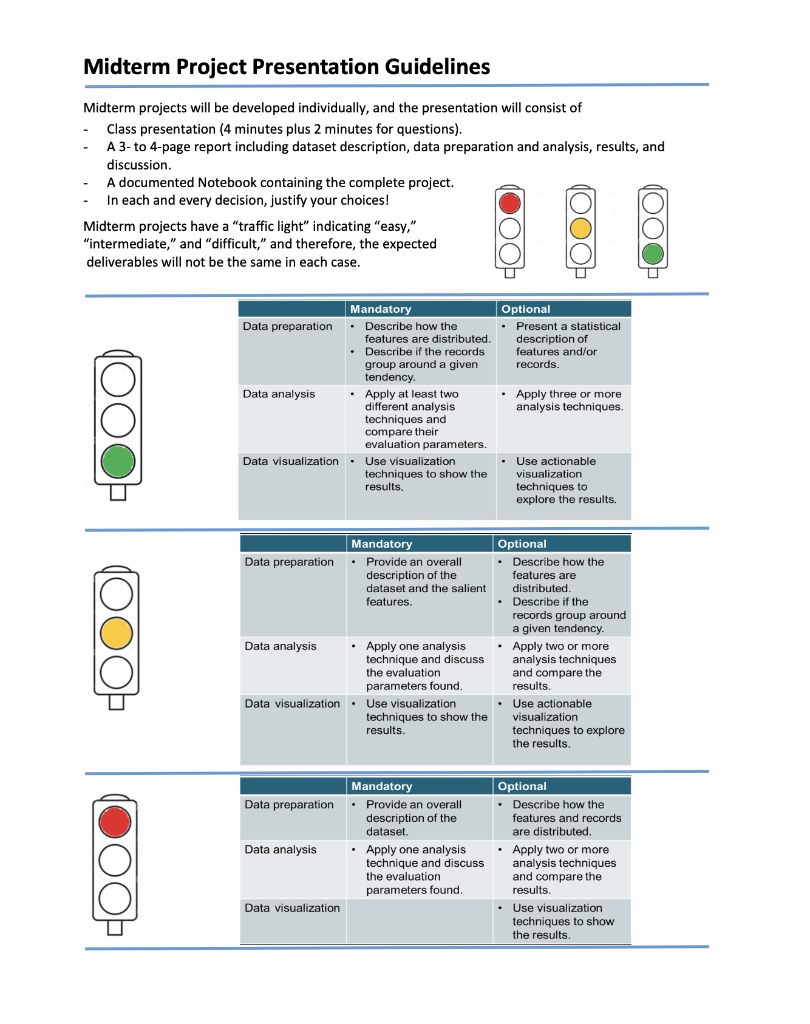
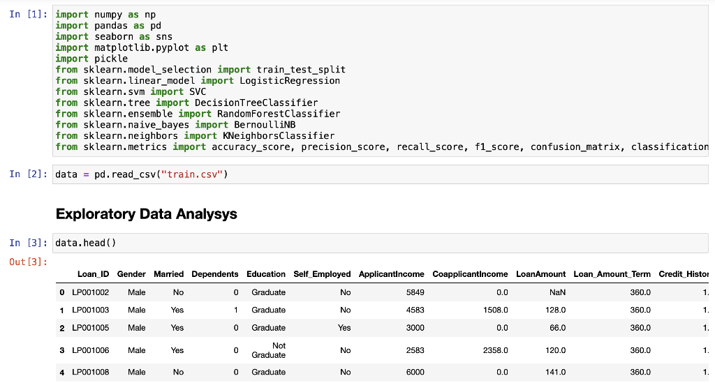
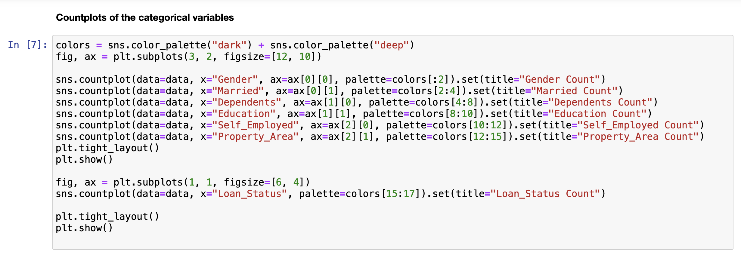
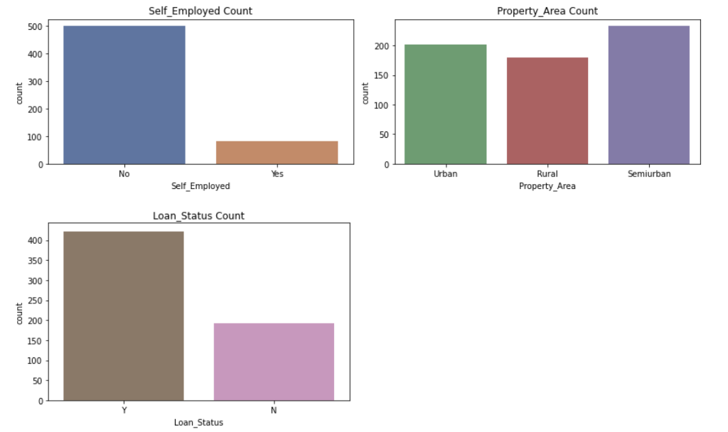
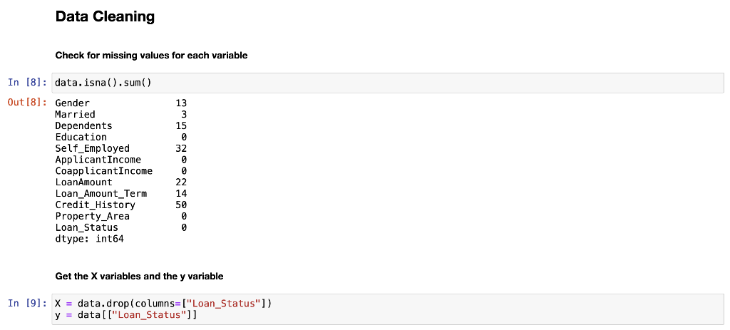
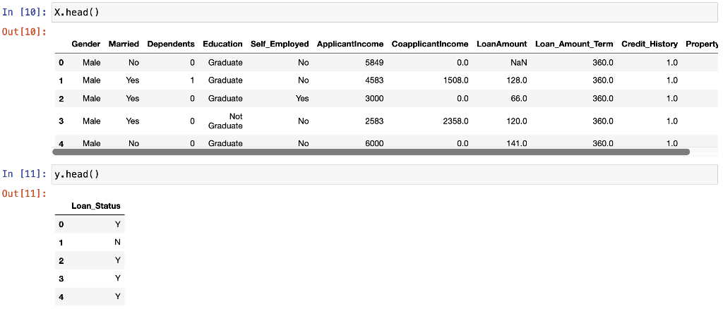
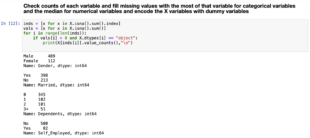
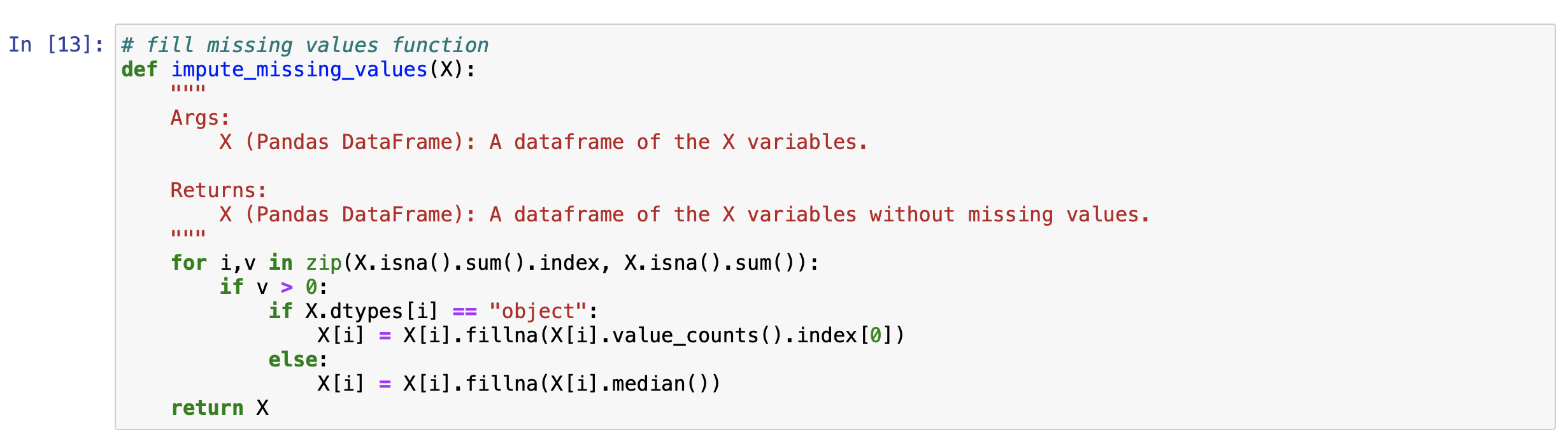
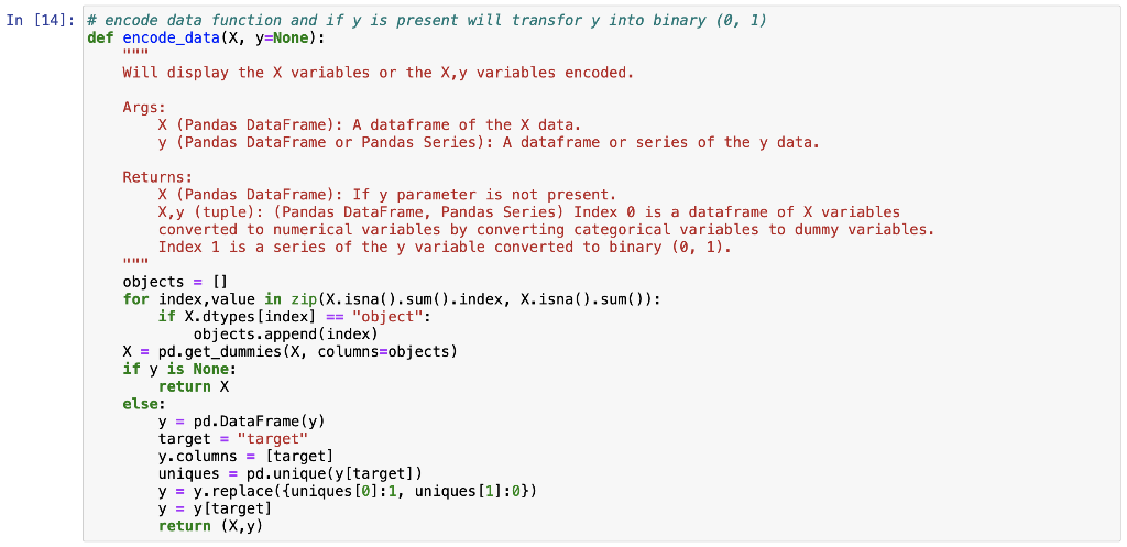
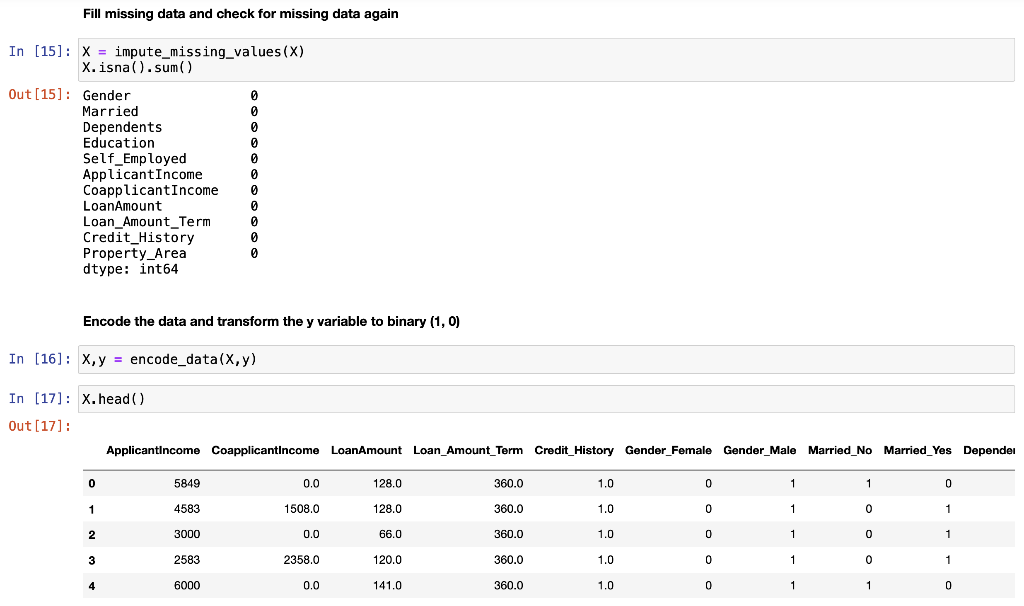
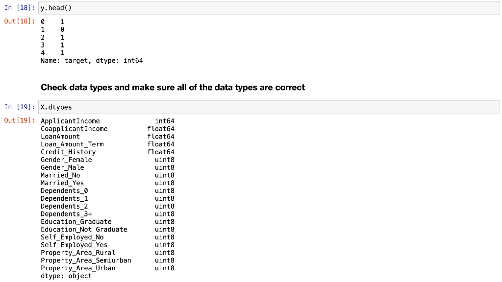
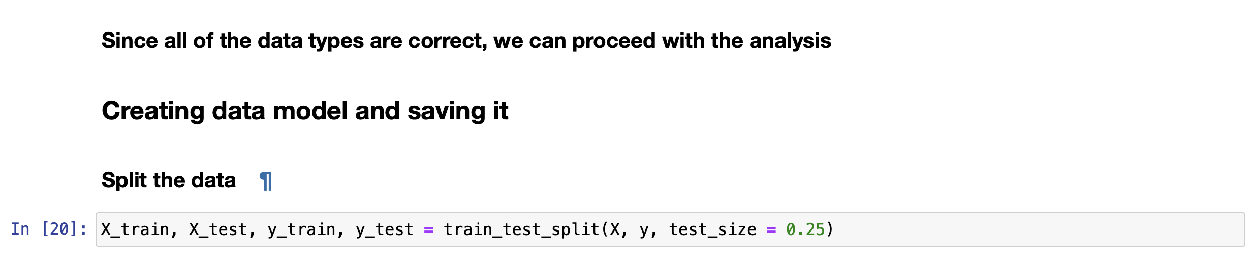
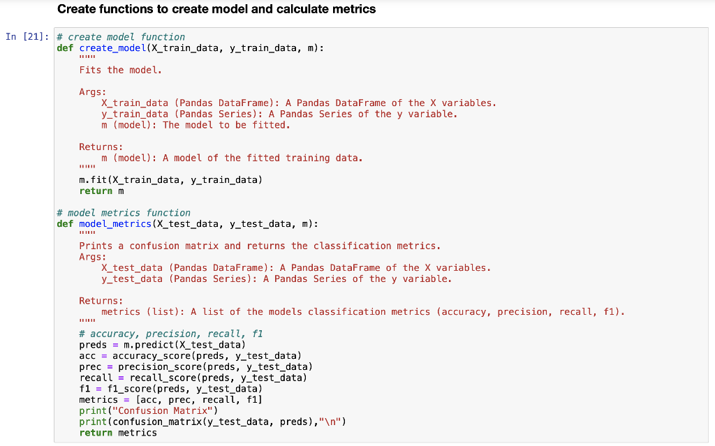
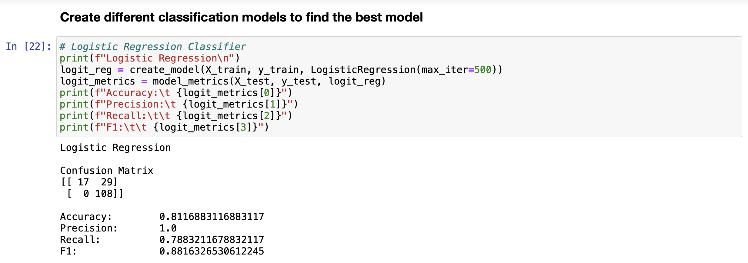
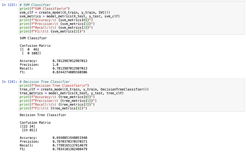
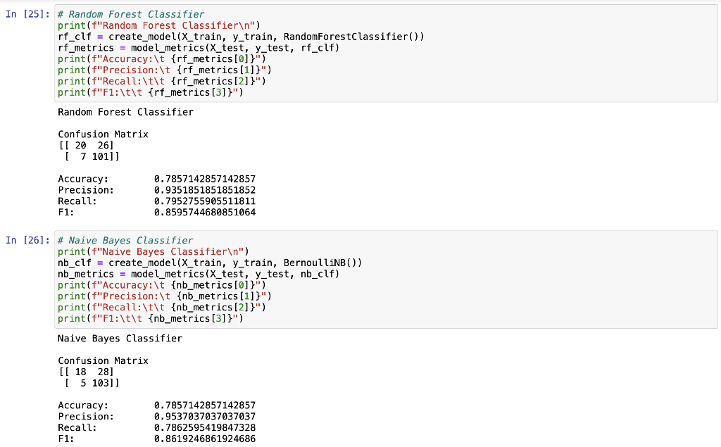
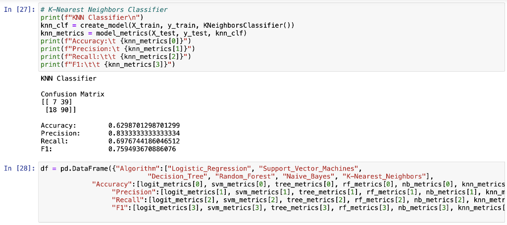
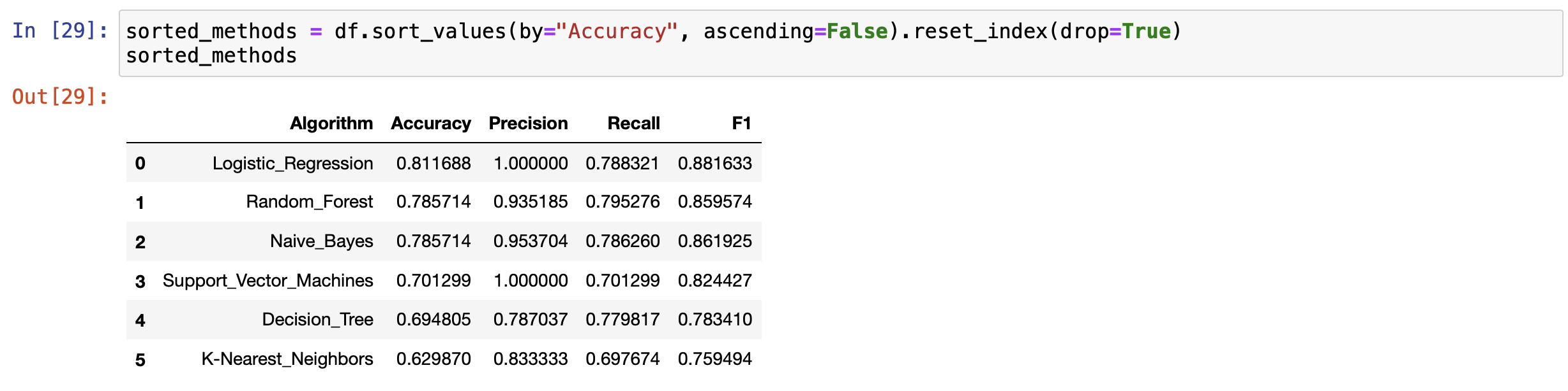
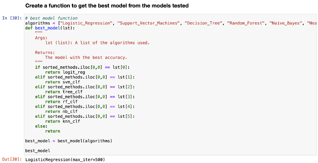
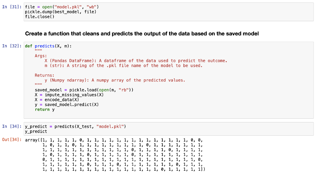
Midterm Project Presentation Guidelines Midterm projects will be developed individually, and the presentation will consist of Class presentation (4 minutes plus 2 minutes for questions). A 3-to 4-page report including dataset description, data preparation and analysis, results, and discussion. A documented Notebook containing the complete project. In each and every decision, justify your choices! Midterm projects have a "traffic light" indicating "easy," "intermediate," and "difficult," and therefore, the expected deliverables will not be the same in each case. loo Optional Present a statistical description of features and/or records. Mandatory Data preparation Describe how the features are distributed. Describe if the records group around a given tendency. Data analysis Apply at least two different analysis techniques and compare their evaluation parameters. Data visualization Use visualization techniques to show the results. Apply three or more analysis techniques Use actionable visualization techniques to explore the results. Mandatory Data preparation Provide an overall description of the dataset and the salient features Data analysis Apply one analysis technique and discuss the evaluation parameters found Data visualization Use visualization techniques to show the results. Optional Describe how the features are distributed Describe if the records group around a given tendency. Apply two or more analysis techniques and compare the results. Use actionable visualization techniques to explore the results. Mandatory Data preparation - Provide an overall description of the dataset. Data analysis Apply one analysis technique and discuss the evaluation parameters found Data visualization Optional Describe how the features and records are distributed. Apply two or more analysis techniques and compare the results. Use visualization techniques to show the results In [1]: import numpy as np import pandas as pd import seaborn as sns import matplotlib.pyplot as plt import pickle from sklearn.model_selection import train_test_split from sklearn. linear_model import LogisticRegression from sklearn.svm import SVC from sklearn. tree import DecisionTreeClassifier from sklearn.ensemble import RandomForestClassifier from sklearn.naive_bayes import BernoulliNB from sklearn.neighbors import KNeighborsClassifier from sklearn.metrics import accuracy_score, precision_score, recall_score, f1_score, confusion_matrix, classification In [2] : data = pd. read_csv("train.csv") 2 Exploratory Data Analysys In [3]: data.head() Out (3]: Loan_ID Gender Married Dependents Education Self Employed Applicantlncome Coapplicantlncome LoanAmount Loan_Amount_Term Credit_Histor 0 LP001002 Male No 0 Graduate No 5849 0.0 NaN 360.0 1. 1 LP001003 Male Yes 1 Graduate No 4583 1508.0 128.0 360.0 1. 2 LPO01005 Male Yes 0 Graduate Yes 3000 0.0 66.0 360.0 1. 3 LPO01006 Male Yes 0 Not Graduate No 2583 2358.0 120.0 360.0 1. 4 LPO01008 Male No 0 Graduate No 6000 0.0 141.0 360.0 1. In [4]: data = data.drop(columns="Loan_ID") In [5]: data.info().
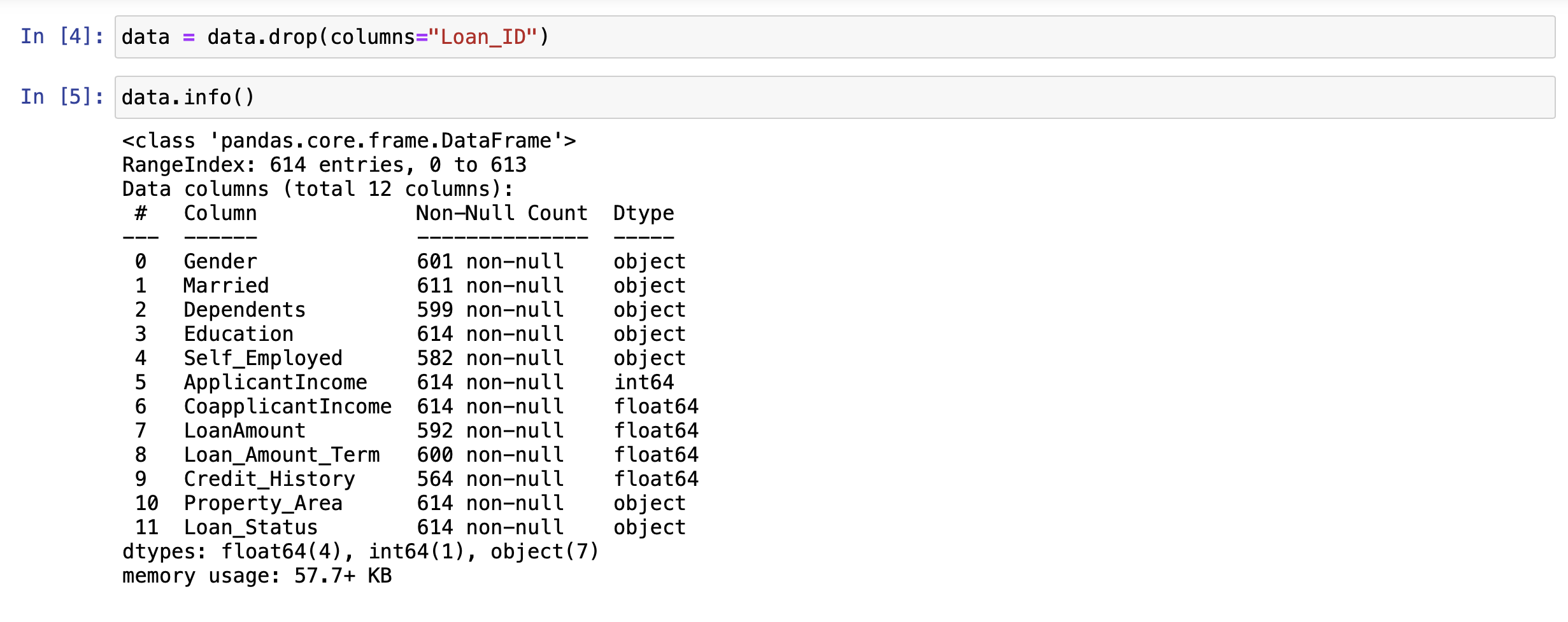
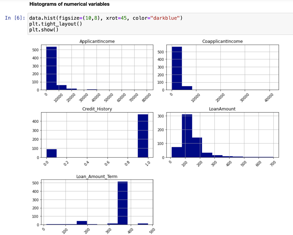
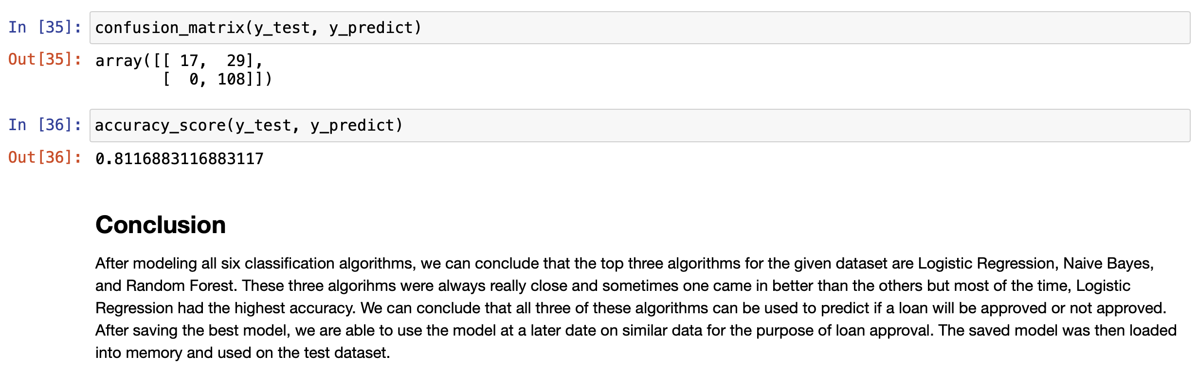
RangeIndex: 614 entries, 0 to 613 Data columns (total 12 columns): # Column Non-Null Count Dtype ON Gender 601 non-null 1 Married 611 non-null 2 Dependents 599 non-null 3 Education 614 non-null 4 Self_Employed 582 non-null 5 Applicant Income 614 non-null 6 CoapplicantIncome 614 non-null 7 LoanAmount 592 non-null 8 Loan_Amount_Term 600 non-null 9 Credit_History 564 non-null 10 Property_Area 614 non-null 11 Loan_Status 614 non-null dtypes: float64(4), int64(1), object(7) memory usage: 57.7+ KB object object object object object int64 float64 float64 float64 float64 object object Histograms of numerical variables In [6]: data.hist(figsize=(10,8), xrot=45, color="darkblue") plt. tight_layout() plt.show() Applicantincome Coapplicantincome 500 400 500 400 300 300 200 200 100 100 0 0 40000 50000 70000 10000 20000 10000 20000 30000 60000 80000 30000 40000 Credit_History LoanAmount 300 400 300 200 EL 200 100 100 0 0 0 0.0 02 200 500 600 700 Loan_Amount_Term 500 400 300 200 100 0 0 100 300 500 Countplots of the categorical variables In [7]: colors = sns.color_palette("dark") + sns.color_palette("deep") " fig, ax = plt. subplots (3, 2, figsize=[12, 10]) = sns.countplot(data=data, x="Gender", ax=ax[0][0], palette=colors[:2]).set(title="Gender Count") sns.countplot(data=data, x="Married", ax=ax [0][1], palette=colors [2:4]).set(title="Married Count") sns.countplot(data=data, x="Dependents", ax=ax[1][0], palette=colors [4:8]).set(title="Dependents Count") sns.countplot(data=data, x="Education", ax=ax[1][1], palette=colors [8:10]).set(title="Education Count") sns.countplot(data=data, x="Self_Employed", axrax [2][0], palette=colors [10:12]).set(title="Self_Employed Count") sns.countplot(data=data, x="Property_Area", ax=ax [2][1], palette=colors [12:15]).set(title="Property_Area Count") plt.tight_layout() plt.show() 1 fig, ax = plt.subplots(1, 1, figsize=[6, 4]) sns.countplot(data=data, x="Loan_Status", palette=colors [15:17]).set(title="Loan_Status Count") plt. tight_layout() plt.show() Gender Count Married Count 500 400 400 300 300 200 200 100 100 0 0 Male Female No Yes Gender Married Dependents Count Education Count 350 500 300 400 250 300 200 count count 150 200 100 100 50 0 0 3+ Graduate Not Graduate Dependents Education Self_Employed Count Property Area Count 500 200 400 150 300 count count 200 100 100 50 0 No Yes Urban Semiurban Self Employed Rural Property Area Loan Status Count 400 350 300 250 count 200 150 100 50 O N Loan_Status Data Cleaning Check for missing values for each variable 13 3 15 0 52 32 In [8]: data. isna().sum() Out [8]: Gender Married Dependents Education Self_Employed Applicant Income Income LoanAmount Loan_Amount_Term Credit_History Property Area Loan_Status dtype: int64 22 14 50 0 0 Get the X variables and the y variable In [9]: X = data.drop(columns=["Loan_Status"]) y = data[("Loan_Status"]] In [10]: X.head() Out [10]: Gender Married Dependents Education Self_Employed Applicantincome Coapplicantincome LoanAmount Loan_Amount_Term Credit_History Property 0 Male No 0 Graduate No 5849 0.0 NaN 360.0 1.0 1 Male Yes 1 Graduate No 4583 1508.0 128.0 360.0 1.0 2 Male Yes 0 Graduate Yes 3000 0.0 66.0 360.0 1.0 3 Male Yes 0 Not Graduate No 2583 2358,0 120.0 360.0 1.0 4 Male No 0 Graduate No 6000 0.0 141.0 360.0 1.0 In [11]: y.head() Out[11]: Loan Status 0 Y 1 N 2 Y 3 Y 4 Y Check counts of each variable and fill missing values with the most of that variable for categorical variables and the median for numerical variables and encode the X variables with dummy variables In [12]: inds = [x for x in X.isna). sum().index] vals = [x for x in X. isna().sum(] for i in range(len(inds)): if vals[i] > 0 and X.dtypes [i] == "object": print(X[inds[i]].value_counts()," ") Male 489 Female 112 Name: Gender, dtype: int64 Yes 398 No 213 Name: Married, dtype: int64 9 345 1 102 2 101 3+ 51 Name: Dependents, dtype: int64 No 500 Yes 82 Name: Self_Employed, dtype: int64 In [13]: # fill missing values function def impute_missing_values(X): IIIIII Args: X (Pandas DataFrame): A dataframe of the X variables. Returns: X (Pandas DataFrame): A dataframe of the X variables without missing values. IIIIII for i,v in zip(X. isna().sum().index, X. isna().sum()): if v > 0: if X.dtypes[i] "object": X[i] = x[i].fillna(X[i].value_counts ().index[@]) else: X[i] X[i]. fillna (X[i].median()) return X = In [14]: # encode data function and if y is present will transfor y into binary (0, 1) def encode_data(x, y=None): Will display the X variables or the X,y variables encoded. Args: X (Pandas DataFrame): A dataframe of the X data. y (Pandas DataFrame or Pandas Series): A dataframe or series of the y data. Returns: X (Pandas DataFrame): If y parameter is not present. X,y (tuple): (Pandas DataFrame, Pandas Series) Index 0 is a dataframe of X variables converted to numerical variables by converting categorical variables to dummy variables. Index 1 is a series of the y variable converted to binary (0, 1). objects = for index, value in zip(X. isna().sum(). index, X. isna().sum()): if X.dtypes [index] == "object": objects.append(index) X = pd.get_dummies (X, columns=objects) if y is None: return X else: = pd.DataFrame(y) target = "target" y.columns = [target] uniques = pd.unique(y[target]) y = y.replace({uniques [0]:1, uniques [1]:0}) y = y[target] return (x,y) Fill missing data and check for missing data again In [15] : X = impute_missing_values(X) X. isna().sum() Out [15]: Gender 9 Married 0 Dependents a Education 0 Self_Employed 0 Applicant Income 0 Coapplicant Income 0 LoanAmount 0 Loan_Amount_Term 0 Credit_History Property_Area dtype: int64 Encode the data and transform the y variable to binary (1, 0) In [16]: X, y = encode_data(x,y) In [17]: X. head() Out [17] : Applicantincome CoapplicantIncome LoanAmount Loan_Amount_Term Credit_History Gender_Female Gender_Male Married_No Married_Yes Depender 0 5849 0.0 128.0 360.0 1.0 0 1 1 0 1 4583 1508.0 128.0 360.0 1.0 0 1 0 o 1 2 3000 0.0 66.0 360.0 1.0 0 1 0 1 3 2583 2358.0 120.0 360.0 1.0 0 0 1 0 1 4 6000 0.0 141.0 360.0 1.0 0 0 1 1 0 In [18]: y.head() Out [18] : 0 1 1 0 2 1 3 4 1 Name: target, dtype: int64 Check data types and make sure all of the data types are correct int64 In [19]: X.dtypes Out (19]: Applicant Income Coapplicant Income LoanAmount Loan Loan_Amount_Term Credit_History Gender_Female Sande Gender Male SMS Married_No MAIS Married_Yes hendes Dependents Dependents Dependents_2 bependents Dependents_3+ Education Graduate Education_Not Graduate Self_Employed_No Self_Employed Yes Property_Area Rural Property Area Semiurban Property Area_Urban dtype: object float64 float64 float64 Calot float64 unto uint8 uint8 who uint8 who uint8 uint8 8 ho uint8 co uint8 ho uint8 uint8 uint8 uint8 uint8 uint8 uint8 uint8 Since all of the data types are correct, we can proceed with the analysis Creating data model and saving it Split the data 1 In [20]: X_train, X_test, y_train, y_test = train_test_split(x, y, test_size = 0.25) 1 Create functions to create model and calculate metrics In [21] : # create model function def create_model(X_train_data, y_train_data, m): Fits the model. Args : X_train_data (Pandas DataFrame): A Pandas DataFrame of the X variables. y_train_data (Pandas Series): A Pandas Series of the y variable. m (model): The model to be fitted. Returns: m (model): A model of the fitted training data. m.fit(X_train_data, y_train_data) return m # model metrics function def model_metrics (X_test_data, y_test_data, m): Prints a confusion matrix and returns the classification metrics. Args: x_test_data (Pandas DataFrame): A Pandas DataFrame of the X variables. y_test_data (Pandas Series): A Pandas Series of the y variable. Returns: metrics (list): A list of the models classification metrics (accuracy, precision, recall, f1). # accuracy, precision, recall, fi preds = m.predict(X_test_data) acc = accuracy_score(preds, y_test_data) prec = precision_score(preds, y_test_data) recall = recall_score(preds, y_test_data) f1 = f1_score(preds, y_test_data) metrics = [acc, prec, recal, f1] print("Confusion Matrix") print(confusion_matrix(y_test_data, preds)," ") return metrics Create different classification models to find the best model In [22]: # Logistic Regression Classifier print(f"Logistic Regression ") logit_reg = create_model(X_train, y_train, LogisticRegression (max_iter=500)) logit_metrics = model_metrics (X_test, y_test, logit_reg) print(f"Accuracy:\t {logit_metrics [0]}") print(f"Precision:\t {logit_metrics [1]}") print(f"Recall:\t\t {logit_metrics [2]}") print("F1:\t\t {logit_metrics [3]}") Logistic Regression Confusion Matrix [[ 17 29] [ 0 108]] Accuracy: Precision: Recall: 0.8116883116883117 1.0 0.7883211678832117 0.8816326530612245 F1: In [23]: # SVM Classifier print("SVM Classifier ") svm_clf = create_model(x_train, y_train, SVCO) svm_metrics = model_metrics(X_test, y_test, svm_clf) print("Accuracy:\t {svm_metrics [@]}") print("Precision:\t {svm_metrics [1]}") print("Recall:\t\t {svm_metrics [2]}") print(f"F1: \t\t {svm_metrics [3]}") SVM Classifier Confusion Matrix [046] [108]] Accuracy: Precision: Recall: F1: 0.7012987012987013 1.0 0.7012987012987013 0.8244274809160306 In [24]: # Decision Tree Classifier print(f"Decision Tree Classifier ") tree_clf = create_model(X_train, y_train, DecisionTreeClassifier()) tree_metrics = model_metrics (X_test, y_test, tree_clf) print("Accuracy:\t {tree_metrics [0]}") print("Precision:\t {tree_metrics [1]}") print("Recall:\t\t {tree_metrics [2]}") print(f"F1:\t\t {tree_metrics [3]}") Decision Tree Classifier Confusion Matrix [[22 24] [23 85] ] Accuracy: Precision: Recall: F1: 0.6948051948051948 0.7870370370370371 0.7798165137614679 0.7834101382488479 In [25]: # Random Forest Classifier print(f"Random Forest Classifier ") rf_clf = create_model(X_train, y_train, RandomForestClassifier() rf_metrics = model_metrics (X_test, y_test, rf_clf) print(f"Accuracy: \t {rf_metrics[0]}") print("Precision:\t {rf_metrics [1]}") print("Recall:\t\t {rf_metrics [2]}") print(f"F1:\t\t {rf_metrics [3]}") Random Forest Classifier Confusion Matrix [[ 20 26] [ 7 101]] Accuracy: Precision: Recall: F1: 0.7857142857142857 0.9351851851851852 0.7952755905511811 0.8595744680851064 In [26]: # Naive Bayes Classifier print("Naive Bayes Classifier ") nb_clf = create_model(X_train, y_train, BernoulliNBO)) nb_metrics = model_metrics (X_test, y_test, nb_clf) print("Accuracy:\t {nb_metrics [0]}") print("Precision:\t {nb_metrics [1]}") print("Recall:\t\t {nb_metrics [2]}") print(f"F1:\t\t {nb_metrics [3]}") Naive Bayes Classifier Confusion Matrix [ 18 28] [ 5 103]] Accuracy: Precision: Recall: F1: 0.7857142857142857 0.9537037037037037 0.7862595419847328 0.8619246861924686 In [27]: # K-Nearest Neighbors Classifier print("KNN Classifier ") knn_clf = create_model(X_train, y_train, kNeighbors Classifier() knn_metrics = model_metrics (X_test, y_test, knn_clf) print(f"Accuracy:\t {knn_metrics [0]}") print("Precision:\t {knn_metrics [1]}") print(f"Recall:\t\t {knn_metrics [2]}") print(f"F1:\t\t {knn_metrics [3]}") KNN Classifier Confusion Matrix [[ 7 39] (18 9011 Accuracy: Precision: Recall: F1: 0.6298701298701299 0.8333333333333334 0.6976744186046512 0.759493670886076 In [28]: df = pd. DataFrame({"Algorithm": ["Logistic_Regression", "Support_Vector_Machines", "Decision-Tree", "Random_Forest", "Naive_Bayes", "K-Nearest Neighbors"), "Accuracy":[logit_metrics[0], svm_metrics [0], tree_metrics [0], rf_metrics[o], nb_metrics[@], knn_metrics "Precision": [logit_metrics[1], sym_metrics [1], tree_metrics [1], rf_metrics [1], nb_metrics [1], knn_m "Recall": [logit_metrics [2], sym_metrics [2], tree_metrics [2], rf_metrics [2], nb_metrics [2], knn_metr "F1": [logit_metrics(3), svm_metrics (3), tree_metrics(3), rf_metrics(3), nb_metrics [3], knn_metrics In [29]: sorted_methods = df.sort_values (by="Accuracy", ascending=False).reset_index(drop=True) sorted_methods Out [29]: Algorithm Accuracy Precision Recall F1 0 Logistic_Regression 0.811688 1.000000 0.788321 0.881633 1 Random_Forest 0.785714 0.935185 0.795276 0.859574 2 Naive_Bayes 0.785714 0.953704 0.786260 0.861925 3 Support_Vector_Machines 0.701299 1.000000 0.701299 0.824427 4 Decision_Tree 0.694805 0.787037 0.779817 0.783410 5 K-Nearest_Neighbors 0.629870 0.833333 0.697674 0.759494 Create a function to get the best model from the models tested In [30] : # best model function algorithms = ("Logistic_Regression", "Support_Vector_Machines", "Decision_Tree", "Random_Forest", "Naive_Bayes", "Nea def best_model(lst): Args: Lst (list): A list of the algorithms used. Returns: The model with the best accuracy. if sorted_methods. iloc[0,0] == lst[0]: return logit_reg elif sorted_methods.iloc[0,0] == Ist[1]: return svm_clf elif sorted_methods.iloc[0,0] == lst (2]: return tree_clf elif sorted_methods.iloc[0,0] == 1st [3]: return rf_clf elif sorted_methods. iloc[0,0] == lst (4): return nb_clf elif sorted_methods.iloc [0,0] == lst [5]: return knn_clf else: return best_model = best_model(algorithms) best_model Out [30]: LogisticRegression (max_iter=500) In [31]: file = open("model.pkl", "wb") pickle. dump(best_model, file) file.close() Create a function that cleans and predicts the output of the data based on the saved model In [32]: def predicts(x, m): Args: X (Pandas DataFrame): A dataframe of the data used to predict the outcome. m (str): A string of the .pkl file name of the model to be used. Returns: y (Numpy ndarray): A numpy array of the predicted values. saved_model = pickle.load(open(m, "rb")) X = impute_missing_values(X) X = encode_data(X) y = saved_model.predict(X) return y In [34]: y_predict = predicts(x_test, "model.pkl") y_predict Out[34]: array([1, 1, 1, 1, 1, 0, 1, 1, 1, 1, 1, 1, 1, 1, 1, 1, 1, 1, 1, 1, 0, 0, 1, 0, 1, 1, 0, 1, 1, 1, 1, 1, 1, 1, 1, 1, 0, 1, 1, 1, 1, 1, 1, 1, 1, 1, 1, 1, 1, 1, 1, 1, 1, 1, 1, 1, 0, 1, 1, 1, 1, 0, 1, 1, 1, 1, 1, 0, 1, 1, 1, 1, 0, 1, 1, 1, 1, 1, 0, 1, 1, 1, 1, 1, 1, 1, 1, 1, 0, 1, 1, 1, 1, 1, 1, 1, 1, 1, 1, 1, 1, 1, 1, 1, 1, 1, 0, 1, 1, 1, 1, 1, 1, 1, 1, 1, 1, 0, 1, 1, 1, 1, 1, 1, 1, 1 1, 1, 0, 1, 1, 1, 1]) In [35]: confusion_matrix(y_test, y_predict) Out [35]: array([[ 17, 29), [ 0, 108]]). In [36]: accuracy_score(y_test, y_predict) Out[36]: 0.8116883116883117 Conclusion After modeling all six classification algorithms, we can conclude that the top three algorithms for the given dataset are Logistic Regression, Naive Bayes, and Random Forest. These three algorihms were always really close and sometimes one came in better than the others but most of the time, Logistic Regression had the highest accuracy. We can conclude that all three of these algorithms can be used to predict if a loan will be approved or not approved. After saving the best model, we are able to use the model at a later date on similar data for the purpose of loan approval. The saved model was then loaded into memory and used on the test dataset