

Answered step by step
Verified Expert Solution
Question
1 Approved Answer
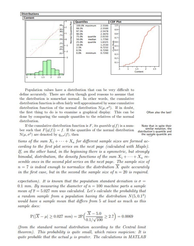
Distributions Content Quantiles CDF Plot .99- 100.0% maximum 2.5500 1.0 -2 99.5%% 2.5500 97.5%% 2.5478 0.9- Normal Quantile Plot -1 .75- 90.0% 2.3070 0.8- 75.0%
Step by Step Solution
There are 3 Steps involved in it
Step: 1

Get Instant Access to Expert-Tailored Solutions
See step-by-step solutions with expert insights and AI powered tools for academic success
Step: 2

Step: 3
Ace Your Homework with AI
Get the answers you need in no time with our AI-driven, step-by-step assistance
Get Started
Mathematical Interest Theory
Authors: Leslie Jane, James Daniel, Federer Vaaler
3rd Edition
147046568X, 978-1470465681