do not use chat$-$gpt$,$ if u do then skip this question cause i have already tried and it cant do the job. i need help with the code to simulate this:Problem $2$: THE SHALLOW WATER MODEL

You have been provided with the Jupyter Notebook code which you can use to simulate surface gravity waves.

Gravity waves are the waves that you see in a pond when you throw a rock into it$.$ They radiate away

from the source of disturbance in a circular pattern. The analytical form of gravity waves can be found from

the linearised Navier Stokes equation $($see chapter $8\mathrm{.}1-2,$ especially equations $(8\mathrm{.}45)$ and $(8\mathrm{.}49)$ in "Fluid

Mechanics" $($Kundu$,$ Cohen and Dowling, $2016)).$

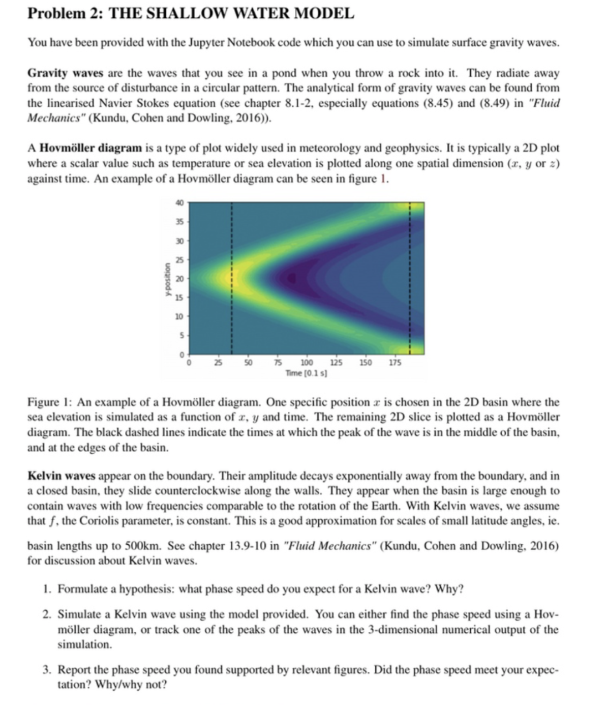
A Hovm$$ller diagram is a type of plot widely used in meteorology and geophysics. It is typically a $2$D plot

where a scalar value such as temperature or sea elevation is plotted along one spatial dimension or $z$

against time. An example of a Hovm$$ller diagram can be seen in figure $1.$

Figure $1$: An example of a Hovm$$ller diagram. One specific position $x$ is chosen in the $2$D basin where the

sea elevation is simulated as a function of $x,y$ and time. The remaining $2$D slice is plotted as a Hovm$$ller

diagram. The black dashed lines indicate the times at which the peak of the wave is in the middle of the basin,

and at the edges of the basin.

Kelvin waves appear on the boundary. Their amplitude decays exponentially away from the boundary, and in

a closed basin, they slide counterclockwise along the walls. They appear when the basin is large enough to

contain waves with low frequencies comparable to the rotation of the Earth. With Kelvin waves, we assume

that $f,$ the Coriolis parameter, is constant. This is a good approximation for scales of small latitude angles, ie$.$

basin lengths up to $500km.$ See chapter $13\mathrm{.}9-10$ in "Fluid Mechanics" $($Kundu$,$ Cohen and Dowling, $2016)$

for discussion about Kelvin waves.

Simulate a Kelvin wave using the model provided. You can either find the phase speed using a Hov$-$

m$$ller diagram, or track one of the peaks of the waves in the $3-$dimensional numerical output of the

simulation.

Report the phase speed you found supported by relevant figures. Did the phase speed meet your expec$-$

tation? Why$/$why not?... code: import numpy as np

from matplotlib import pyplot as plt

from matplotlib import animation

def run$\_$model $($dx$,$ dy$,$ Lx$,$ Ly$,$ eta$0,$ f$0,$ beta, Kelvin$=$False, Rossby$=$False, Nt$=100000)$:

# define slices

M $=$ slice$(1,-1)$

L $=$ slice$(0,-2)$

R $=$ slice$(2,$ None$)$

# define difference functions

def Dx$0($h$,$ dx$)$:

return $1/$dx $*($h$[$R$,$M$]-$ h$[$M$,$M$])$

def Dx$1($u$,$ dx$)$:

return $1/$dx $*($u$[$M$,$M$]-$ u$[$L$,$M$])$

def Dy$0($h$,$ dy$)$:

return $1/$dy $*($h$[$M$,$R$]-$ h$[$M$,$M$])$

def Dy$1($v$,$ dy$)$:

return $1/$dy $*($v$[$M$,$M$]-$ v$[$M$,$L$])$

#parameters in SI units

g $=9\mathrm{.}81$

depth $=10.$

epsilon $=0\mathrm{.}01$

c $=$ np$.$sqrt$($g$*$depth$)$

Nx $=$ int$($Lx$/$dx$)$

Ny $=$ int$($Ly$/$dy$)$

dt $=0\mathrm{.}1*$dx$/$c

if Kelvin:

A $=$ dt $*$ f$0$

B $=1/4*$ A $**2$

elif Rossby:

f $=$ np$.$zeros$($Ny$+1)$

A $=$ np$.$zeros$($Ny$+1)$

B $=$ np$.$zeros$($Ny$+1)$

for y in range$($Ny$)$:

f$[$y$]=$ f$0+$ beta $*$ y $*$ dy

A$[$y$]=$ dt $*$ f$[$y$]$

B$[$y$]=1/4*$ A$[$y$]**2$

eta $=$ np$.$zeros$(($Nx$+1,$ Ny$+1))$

eta$3$D $=$ np$.$zeros$(($Nt$+1,$ Nx$+1,$ Ny$+1))$

u $=$ np$.$zeros$(($Nx$+1,$ Ny$+1))$

v $=$ np$.$zeros$(($Nx$+1,$ Ny$+1))$

# initial conditions

eta $=$ eta$0.$copy$()$

t $=0$

cnt $=0$

while cnt