Documentation for CPS08 Data

Each month the Bureau of Labor Statistics in the U.S. Department of Labor conducts the Current Population Survey (CPS), which provides data on labor force characteristics of the population, including the level of employment, unemployment, and earnings. Approximately 65,000 randomly selected U.S. households are surveyed each month. The sample is chosen by randomly selecting addresses from a database comprised of addresses from the most recent decennial census augmented with data on new housing units constructed after the last census. The exact random sampling scheme is rather complicated (first small geographical areas are randomly selected, then housing units within these areas randomly selected); details can be found in the Handbook of Labor Statistics and is described on the Bureau of Labor Statistics website (www.bls.gov).

The survey conducted each March is more detailed than in other months and asks questions about earnings during the previous year. The file CPS08 contains the data for 2008 (from the March 2009 survey). These data are for full-time workers, defined as workers employed more than 35 hours per week for at least 48 weeks in the previous year. Data are provided for workers whose highest educational achievement is (1) a high school diploma, and (2) a bachelors degree. Series in Data Set:

FEMALE: 1 if female, 0 if male YEAR: year AHE : average hourly earning BACHELOR: 1 if worker has a bachelors degree; 0 if worker has a high school degree

CPS08

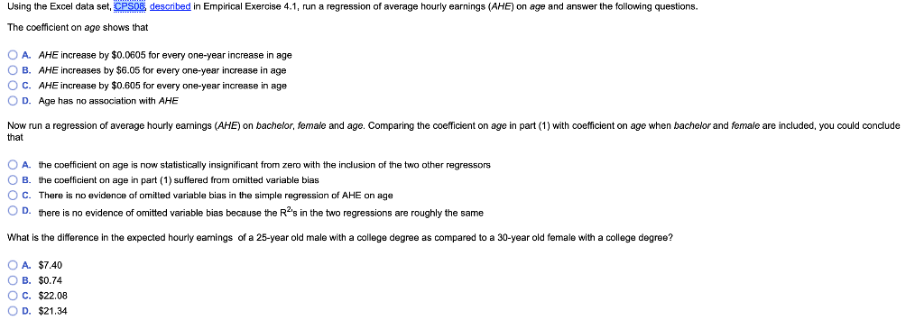
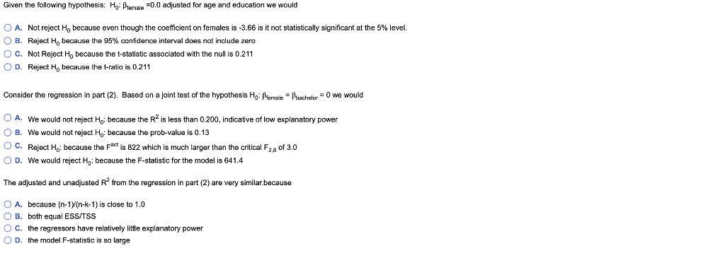
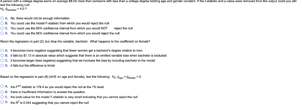
Using the Excel data set, CPSO8 descibed in Empirica.1, run a regression of average hourly earnings (AHE) on age and answer the following questions. The coefficient on age shows that OA. AHE increase by $0.0605 for every one-year increase in age O B. AHE increases by $6.05 for every one-year increase in age O c. AHE increase by $0.605 for every one-year increase in age O D. Age has no association with AHE Now run a regression of average hourly earnings (AHE) on bachelor, female and age. Comparing the coefficient on age in part (1) with coefficient on age when bachelor and female are included, you could conclude that OA. the coefficient on age is now statistically insignificant from zero with the inclusion of the two other regressors O B. the coefficient on age in part (1) suffered from omitted variable bias O C. There is no evidence of omitted variable bias in the simple regression of AHE on age OD. there is no evidence of omitted variable bias because the R2's in the two regressions are roughly the same What is the difference in the expected hourly eamings of a 25-year old male with a college degree as compared to a 30-year old female with a college degree? OA. $7.40 OB. $0.74 O C. $22.08 D. $21.34 Given the following hypothesis: Hai Premale -0.0 adjusted for age and education we would O A. Not reject Ho because even though the coefficient on females is 3.66 is it not statistically significant at the 5% level. O B. Reject Ho because the 95% confidence interval does not include zero O C. Not Reject Ho because the t-statistic associated with the null is 0.211 O D. Reject Ho because the t-ratio is 0.211 Consider the regression in part (2). Based on a joint test of the hypothesis Ho: Plemaie-Pachelor-0 we would O A. We would not reject Ho: because the R2 is less than 0.200, indicative of low explanatory power OB. We would not reject Ho: because the prob-value is 0.13 C. Reject Ho' because the Fact is 822 which is much larger than the critical F28 of 3.0 D. We would reject Ho: because the F-statistic for the model is 641.4 The adjusted and unadjusted R" from the regression in part (2) are very similar.because O A. because (n-1)/(n-k-1) is close to 1.0 O B. both equal ESS/TSS O C. the regressors have relatively little explanatory power O D. the model F-statistic is so large Ah a college degree eams on average$8.03 more than someone with less than a college degree holding age and gender cstant. If the t-stalistic and p-value were removed from the output could you stil test the following null : bachelor . 4.0 ? O A. No, there would not be enough information 0 B. You could use the model F-statistic from which you would reject the null C. You could use the 95% confidence interval from which you would NOT reject the null 0 D. You could use the 95% confidence interval from which you would reject the nul Rerun the regression in part (2), but drop the variable, bachelor. What happens to the coefficient on female? O A it becomes more negative suggesting that fewer women get a bachelor's degree relative to men B. it falls by $1.13 in absolute value which suggests that there is an omitted variable bias when bachelor is excluded O C. it becomes larger (less negative) suggesting that we increase the bias by including bachelor in the model 0 D. it falls but the difference is trivial Based on the regression in part (8) (AHE on age and female), test the following: H PagePtomale0. A, the Fact statistic is 1784 so you would reject the null at the 1% level 0 B. there is insufficient information to answer the question C. the prob value for the model F-statistic is very small indicating that you cannot reject the null 0 D, the R2 is 0.044 suggesting that you cannot reject the null Using the Excel data set, CPSO8 descibed in Empirica.1, run a regression of average hourly earnings (AHE) on age and answer the following questions. The coefficient on age shows that OA. AHE increase by $0.0605 for every one-year increase in age O B. AHE increases by $6.05 for every one-year increase in age O c. AHE increase by $0.605 for every one-year increase in age O D. Age has no association with AHE Now run a regression of average hourly earnings (AHE) on bachelor, female and age. Comparing the coefficient on age in part (1) with coefficient on age when bachelor and female are included, you could conclude that OA. the coefficient on age is now statistically insignificant from zero with the inclusion of the two other regressors O B. the coefficient on age in part (1) suffered from omitted variable bias O C. There is no evidence of omitted variable bias in the simple regression of AHE on age OD. there is no evidence of omitted variable bias because the R2's in the two regressions are roughly the same What is the difference in the expected hourly eamings of a 25-year old male with a college degree as compared to a 30-year old female with a college degree? OA. $7.40 OB. $0.74 O C. $22.08 D. $21.34 Given the following hypothesis: Hai Premale -0.0 adjusted for age and education we would O A. Not reject Ho because even though the coefficient on females is 3.66 is it not statistically significant at the 5% level. O B. Reject Ho because the 95% confidence interval does not include zero O C. Not Reject Ho because the t-statistic associated with the null is 0.211 O D. Reject Ho because the t-ratio is 0.211 Consider the regression in part (2). Based on a joint test of the hypothesis Ho: Plemaie-Pachelor-0 we would O A. We would not reject Ho: because the R2 is less than 0.200, indicative of low explanatory power OB. We would not reject Ho: because the prob-value is 0.13 C. Reject Ho' because the Fact is 822 which is much larger than the critical F28 of 3.0 D. We would reject Ho: because the F-statistic for the model is 641.4 The adjusted and unadjusted R" from the regression in part (2) are very similar.because O A. because (n-1)/(n-k-1) is close to 1.0 O B. both equal ESS/TSS O C. the regressors have relatively little explanatory power O D. the model F-statistic is so large Ah a college degree eams on average$8.03 more than someone with less than a college degree holding age and gender cstant. If the t-stalistic and p-value were removed from the output could you stil test the following null : bachelor . 4.0 ? O A. No, there would not be enough information 0 B. You could use the model F-statistic from which you would reject the null C. You could use the 95% confidence interval from which you would NOT reject the null 0 D. You could use the 95% confidence interval from which you would reject the nul Rerun the regression in part (2), but drop the variable, bachelor. What happens to the coefficient on female? O A it becomes more negative suggesting that fewer women get a bachelor's degree relative to men B. it falls by $1.13 in absolute value which suggests that there is an omitted variable bias when bachelor is excluded O C. it becomes larger (less negative) suggesting that we increase the bias by including bachelor in the model 0 D. it falls but the difference is trivial Based on the regression in part (8) (AHE on age and female), test the following: H PagePtomale0. A, the Fact statistic is 1784 so you would reject the null at the 1% level 0 B. there is insufficient information to answer the question C. the prob value for the model F-statistic is very small indicating that you cannot reject the null 0 D, the R2 is 0.044 suggesting that you cannot reject the null