dont worry about extra credit.
Some code is provided so fill in what is needed
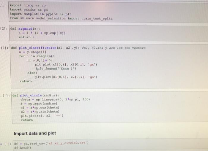
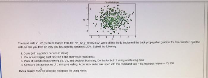
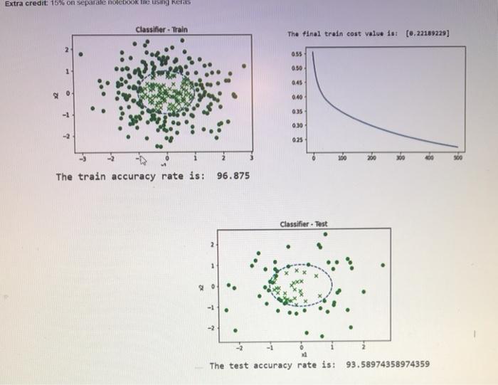
Class Output The input data x1, x2, y can be loaded from file: "x1x2y_circle2.csv" Work of this file to implement the back propagation gradient for this classifier. Sple the data so that you train on 80% and test with the remaining 20% Submit the following 1. Code (with algorithm derived in class) 2 Plot of converging cost function and final value (train data) 3. Plots of classification showing is, o's, and decision boundary. Do this for both training and testing data 4. Compare the accuracies of training vs desting Accuracy can be calcuated with this command accnp mean(nprint(A) - Y*100 Extra credit: 15/16 on separate notebook file using keras Extra credit: 15% on separate notebook using Relas Classifier - Train The final train cost value is: (0.22189229] 0.55 0.30 0:45 040 0.30 100 18 8 18 The train accuracy rate is: 96.875 Classifier. Test 2 OK -1 -2 The test accuracy rate is: 93.58974358974359 [1] : import numpy as np import pandas as pd import matplotlib.pyplot as pit from sklearn.model_selection Import train teat_split [2]: def sigmoid(s): a - 1 / (1+ np.exp(--)) returna (3): def plot_classification (x1, x2 .y): #x1, x2, and y are ixm row vectors m - y.shape (1) for i in range (m): if y[0, 1]>.5: plt.plot(x1(0,1). x20,1), 'gx') #plt. legend('Exam 1') else: plt.plot(x110, 11, x2[0,1], 'go) return [1: det plot_circle (radius): theta - np.linspace(0, 2np.pi, 100) np.sqrt (radius) *i- np.cos(theta) *2- np.sin(theta) plt.plot(x1, x2, I--) return Import data and plot +01: df - pd. read_cav('x1_x2y_circle2.cav') df.head() Class Output The input data x1, x2, y can be loaded from file: "x1x2y_circle2.csv" Work of this file to implement the back propagation gradient for this classifier. Sple the data so that you train on 80% and test with the remaining 20% Submit the following 1. Code (with algorithm derived in class) 2 Plot of converging cost function and final value (train data) 3. Plots of classification showing is, o's, and decision boundary. Do this for both training and testing data 4. Compare the accuracies of training vs desting Accuracy can be calcuated with this command accnp mean(nprint(A) - Y*100 Extra credit: 15/16 on separate notebook file using keras Extra credit: 15% on separate notebook using Relas Classifier - Train The final train cost value is: (0.22189229] 0.55 0.30 0:45 040 0.30 100 18 8 18 The train accuracy rate is: 96.875 Classifier. Test 2 OK -1 -2 The test accuracy rate is: 93.58974358974359 [1] : import numpy as np import pandas as pd import matplotlib.pyplot as pit from sklearn.model_selection Import train teat_split [2]: def sigmoid(s): a - 1 / (1+ np.exp(--)) returna (3): def plot_classification (x1, x2 .y): #x1, x2, and y are ixm row vectors m - y.shape (1) for i in range (m): if y[0, 1]>.5: plt.plot(x1(0,1). x20,1), 'gx') #plt. legend('Exam 1') else: plt.plot(x110, 11, x2[0,1], 'go) return [1: det plot_circle (radius): theta - np.linspace(0, 2np.pi, 100) np.sqrt (radius) *i- np.cos(theta) *2- np.sin(theta) plt.plot(x1, x2, I--) return Import data and plot +01: df - pd. read_cav('x1_x2y_circle2.cav') df.head()