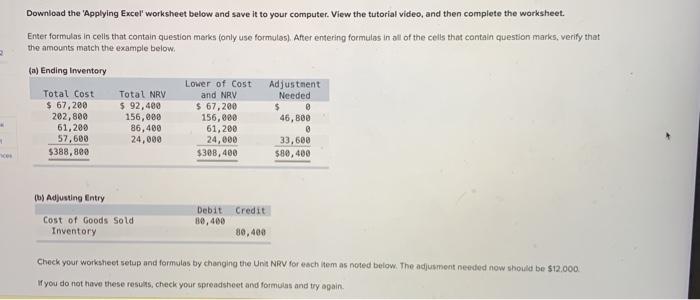
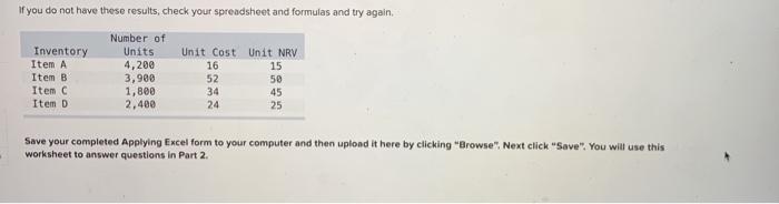
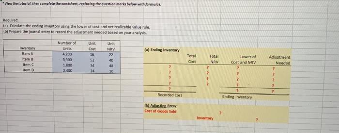
Download the 'Applying Excel' worksheet below and save it to your computer. View the tutorial video, and then complete the worksheet. Enter formulas in cells that contain question marks (only use formulas). After entering formulas in all of the cells that contain question marks, verify that the amounts match the example below. (a) Ending Inventory Total Cost $ 67,200 202,800 61,200 57,600 $388,880 Total NRV 5 92,400 156,000 86,400 24,000 Lower of Cost and NRV $ 67,200 156,000 61,200 24,000 $308,400 Adjustment Needed $ @ 46,800 @ 33,600 $80,400 (1) Adjusting Entry Credit Cost of Goods Sold entory Debit 80,400 80,400 Check your worksheet setup and formulas by changing the Unit NRV for each item as noted below. The adjusment needed now should be $12.000 If you do not have these results, check your spreadsheet and formulas and try again If you do not have these results, check your spreadsheet and formulas and try again. Inventory Item A Item B Item C Item D Number of Units 4,200 3,900 1,800 2,400 Unit Cost Unit NRV 16 15 52 50 34 45 24 25 Save your completed Applying Excel form to your computer and then upload it here by clicking "Browse", Next click "Save". You will use this worksheet to answer questions in Part 2 View the tutorial, then complete the worksheet, replacing the question marks below with formulas. Required (a) Calculate the ending inventory using the lower of cost and net realizable value rule. (b) Prepare the journal entry to record the adjustment needed based on your analysis. Number of Unit Cast (a) Ending Inventory 16 Inventory Item A Item B item Item D 4,200 3.900 1800 2.400 Unit NRV 22 40 48 10 Total Cost Lower of Cast and NRV Adjustment Needed 2 24 7 7 2 Total NRV 7 2 7 ? 7 ? ? 2 7 Ending Inventory 2 2 Recorded Cost El Adjusting Entry Cost of Goods Sold 7 Inventory