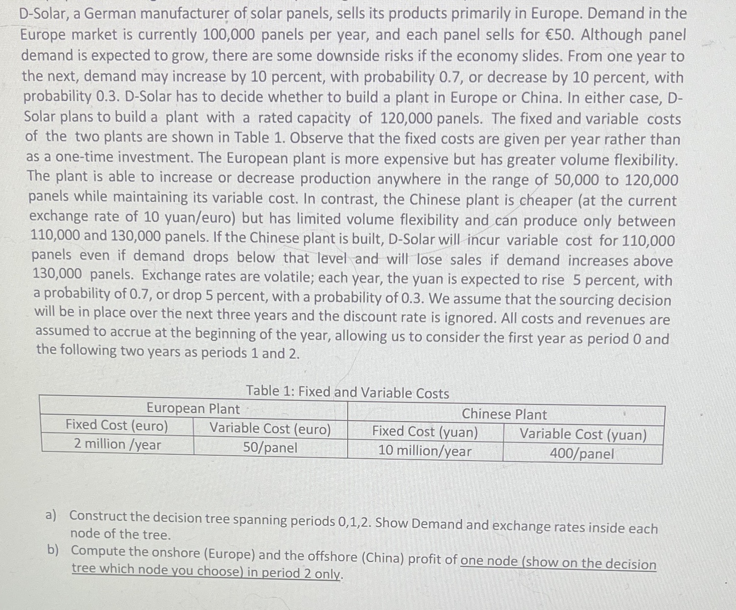
D-Solar, a German manufacturer of solar panels, sells its products primarily in Europe. Demand in the Europe market is currently 100,000 panels per year, and each panel sells for E50. Although panel demand is expected to grow, there are some downside risks if the economy slides. From one year to the next, demand may increase by 10 percent, with probability 0.7, or decrease by 10 percent, with probability 0.3. D-Solar has to decide whether to build a plant in Europe or China. In either case, D- Solar plans to build a plant with a rated capacity of 120,000 panels. The fixed and variable costs of the two plants are shown in Table 1. Observe that the fixed costs are given per year rather than as a one-time investment. The European plant is more expensive but has greater volume flexibility. The plant is able to increase or decrease production anywhere in the range of 50,000 to 120,000 panels while maintaining its variable cost. In contrast, the Chinese plant is cheaper (at the current exchange rate of 10 yuan/euro) but has limited volume flexibility and can produce only between 110,000 and 130,000 panels. If the Chinese plant is built, D-Solar will incur variable cost for 110,000 panels even if demand drops below that level and will lose sales if demand increases above 130,000 panels. Exchange rates are volatile; each year, the yuan is expected to rise 5 percent, with a probability of 0.7, or drop 5 percent, with a probability of 0.3. We assume that the sourcing decision will be in place over the next three years and the discount rate is ignored. All costs and revenues are assumed to accrue at the beginning of the year, allowing us to consider the first year as period 0 and the following two years as periods 1 and 2. Table 1: Fixed and Variable Costs European Plant Chinese Plant Fixed Cost (euro) Variable Cost (euro) Fixed Cost (yuan) Variable Cost (yuan) 2 million /year 50/panel 10 million/year 400/panel a) Construct the decision tree spanning periods 0, 1,2. Show Demand and exchange rates inside each node of the tree. b) Compute the onshore (Europe) and the offshore (China) profit of one node (show on the decision tree which node you choose) in period 2 only


