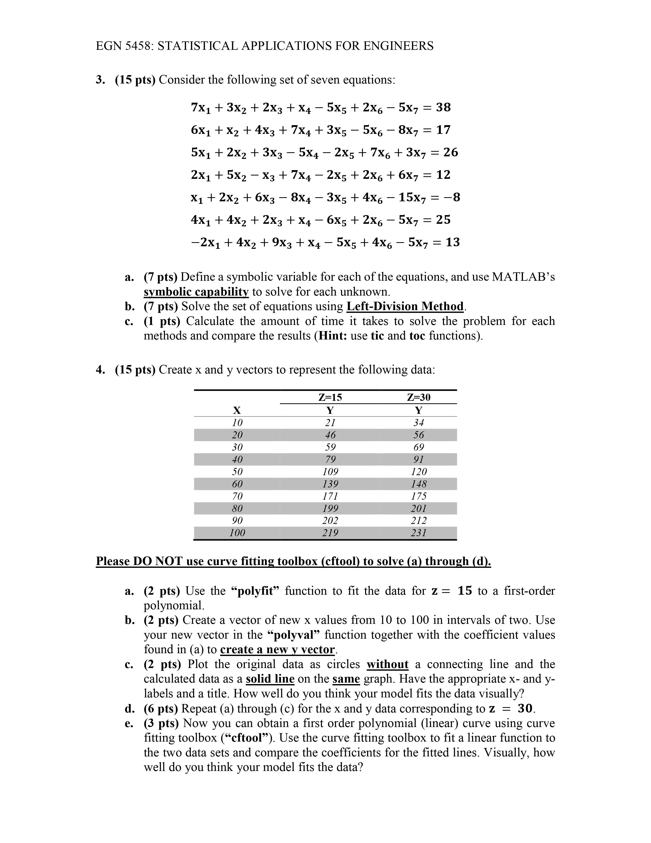
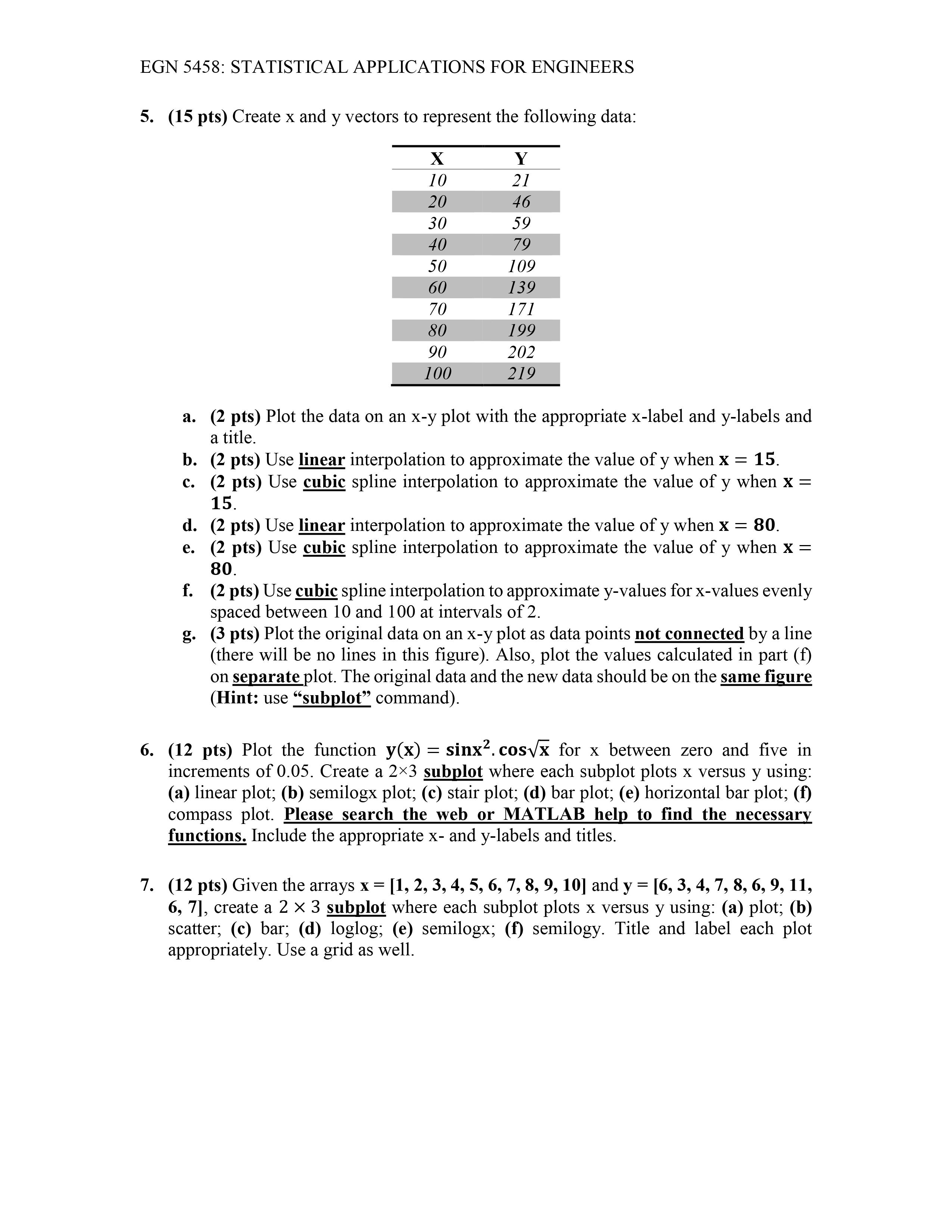
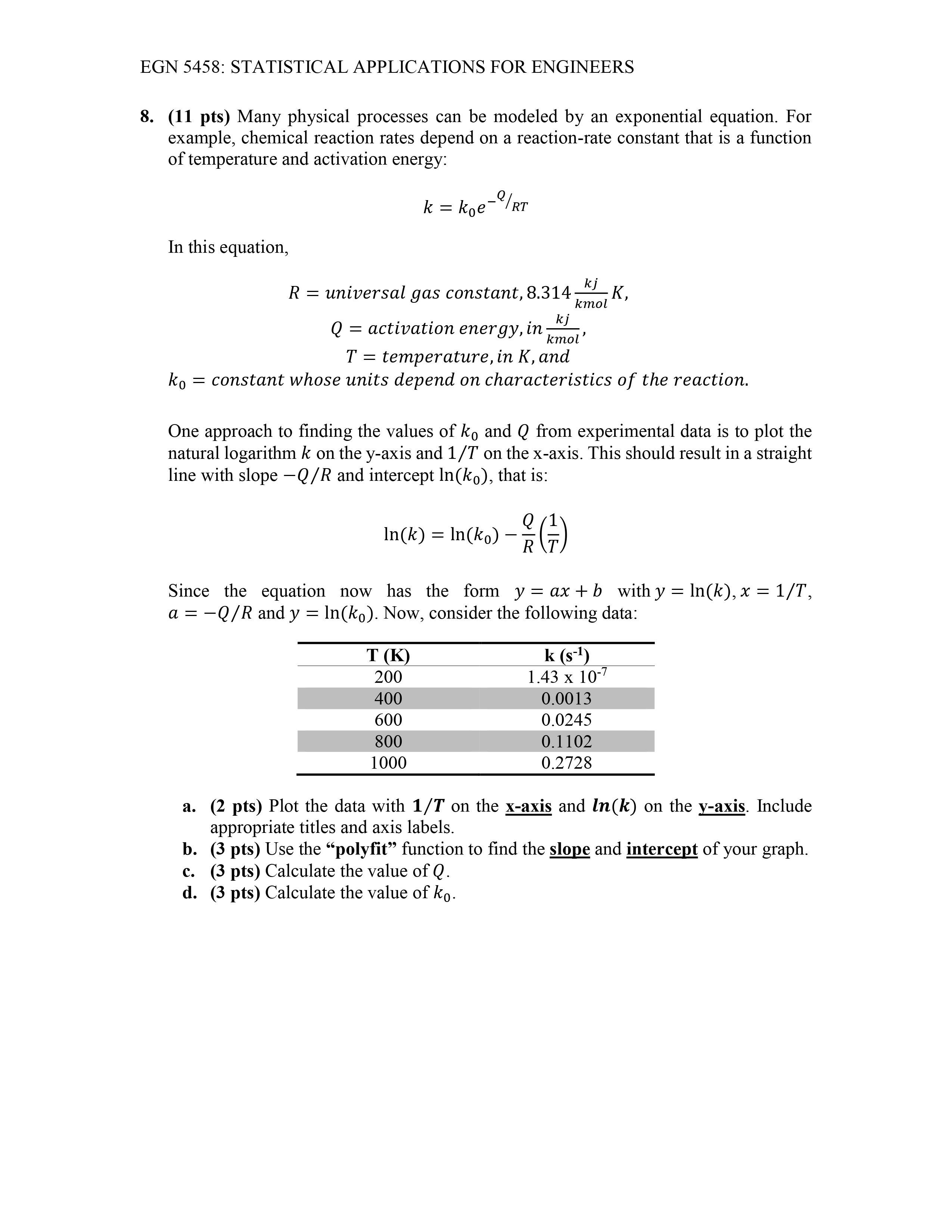
EGN 5458: STATISTICAL APPLICATIONS FOR ENGINEERS HOMEWORK 6 Due: 11.02.2023, 08:00 PM Please submit your homework on CANVAS using the assignment page for Homework 6. Please send your homework in ONE SINGLE, complete, and sorted PDF or Word file. In this homework, please use MATLAB to solve the questions and EMBED YOUR SCRIPT (code) into the text with your submission instead of a separate attachment. MATLAB command window screenshots should show your RUN RESULTS. 1. (10 pts) Determine the first and second derivatives of the following functions, using MATLAB's symbolic functions: a. (2 pts) f1(x)=y=2x45x2+6x+12 b. (2 pts) f2(x)=y=(x34x2+3x+8)(x3) c. (2 pts) f3(x)=y=sin(4x2)cos(6x) d. (2 pts) f4(x)=y=4x2e6x3 e. (2 pts) f5(x)=y=ln(4x2) 2. (10 pts) Use MATLAB's symbolic functions to perform the following integrations: a. (2 pts) f1(x)=y=(3x22x+6x+12) b. (2 pts) f2(x)=y=(x25x+2.8)(x2) c. (2 pts) f3(x)=y=tan(3x2)cos(2x) d. (2 pts) f4(x)=y=5x3e2x4 e. (2 pts) f5(x)=y=ln(2x4) EGN 5458: STATISTICAL APPLICATIONS FOR ENGINEERS 8. (11 pts) Many physical processes can be modeled by an exponential equation. For example, chemical reaction rates depend on a reaction-rate constant that is a function of temperature and activation energy: k=k0eQ/RT In this equation, R=universalgasconstant,8.314kmolkjK,Q=activationenergy,inkmolkj,T=temperature,inK,andk0=constantwhoseunitsdependoncharacteristicsofthereaction. One approach to finding the values of k0 and Q from experimental data is to plot the natural logarithm k on the y-axis and 1/T on the x-axis. This should result in a straight line with slope Q/R and intercept ln(k0), that is: ln(k)=ln(k0)RQ(T1) Since the equation now has the form y=ax+b with y=ln(k),x=1/T, a=Q/R and y=ln(k0). Now, consider the following data: a. (2 pts) Plot the data with 1/T on the x-axis and ln(k) on the y-axis.Include appropriate titles and axis labels. b. (3 pts) Use the "polyfit" function to find the slope and intercept of your graph. c. (3 pts) Calculate the value of Q. d. (3 pts) Calculate the value of k0. EGN 5458: STATISTICAL APPLICATIONS FOR ENGINEERS 3. (15 pts) Consider the following set of seven equations: 7x1+3x2+2x3+x45x5+2x65x7=386x1+x2+4x3+7x4+3x55x68x7=175x1+2x2+3x35x42x5+7x6+3x7=262x1+5x2x3+7x42x5+2x6+6x7=12x1+2x2+6x38x43x5+4x615x7=84x1+4x2+2x3+x46x5+2x65x7=252x1+4x2+9x3+x45x5+4x65x7=13 a. (7 pts) Define a symbolic variable for each of the equations, and use MATLAB's symbolic capability to solve for each unknown. b. (7 pts) Solve the set of equations using Left-Division Method. c. (1 pts) Calculate the amount of time it takes to solve the problem for each methods and compare the results (Hint: use tic and toc functions). 4. (15 pts) Create x and y vectors to represent the following data: Please DO NOT use curve fitting toolbox (cftool) to solve (a) through (d). a. (2 pts) Use the "polyfit" function to fit the data for z=15 to a first-order polynomial. b. (2 pts) Create a vector of new x values from 10 to 100 in intervals of two. Use your new vector in the "polyval" function together with the coefficient values found in (a) to create a new y vector. c. (2 pts) Plot the original data as circles without a connecting line and the calculated data as a solid line on the same graph. Have the appropriate x and y labels and a title. How well do you think your model fits the data visually? d. (6 pts) Repeat (a) through (c) for the x and y data corresponding to z=30. e. (3 pts) Now you can obtain a first order polynomial (linear) curve using curve fitting toolbox ("cftool"). Use the curve fitting toolbox to fit a linear function to the two data sets and compare the coefficients for the fitted lines. Visually, how well do you think your model fits the data? EGN 5458: STATISTICAL APPLICATIONS FOR ENGINEERS 5. (15 pts) Create x and y vectors to represent the following data: a. (2 pts) Plot the data on an xy plot with the appropriate x-label and y-labels and a title. b. (2 pts) Use linear interpolation to approximate the value of y when x=15. c. (2 pts) Use cubic spline interpolation to approximate the value of y when x= 15. d. (2 pts) Use linear interpolation to approximate the value of y when x=80. e. (2 pts) Use cubic spline interpolation to approximate the value of y when x= 80. f. (2 pts) Use cubic spline interpolation to approximate y-values for x-values evenly spaced between 10 and 100 at intervals of 2 . g. (3 pts) Plot the original data on an xy plot as data points not connected by a line (there will be no lines in this figure). Also, plot the values calculated in part (f) on separate plot. The original data and the new data should be on the same figure (Hint: use "subplot" command). 6. (12 pts) Plot the function y(x)=sinx2cosx for x between zero and five in increments of 0.05 . Create a 23 subplot where each subplot plots x versus y using: (a) linear plot; (b) semilogx plot; (c) stair plot; (d) bar plot; (e) horizontal bar plot; (f) compass plot. Please search the web or MATLAB help to find the necessary functions. Include the appropriate x - and y-labels and titles. 7. (12 pts) Given the arrays x=[1,2,3,4,5,6,7,8,9,10] and y=[6,3,4,7,8,6,9,11, 6, 7], create a 23 subplot where each subplot plots x versus y using: (a) plot; (b) scatter; (c) bar; (d) loglog; (e) semilogx; (f) semilogy. Title and label each plot appropriately. Use a grid as well. EGN 5458: STATISTICAL APPLICATIONS FOR ENGINEERS HOMEWORK 6 Due: 11.02.2023, 08:00 PM Please submit your homework on CANVAS using the assignment page for Homework 6. Please send your homework in ONE SINGLE, complete, and sorted PDF or Word file. In this homework, please use MATLAB to solve the questions and EMBED YOUR SCRIPT (code) into the text with your submission instead of a separate attachment. MATLAB command window screenshots should show your RUN RESULTS. 1. (10 pts) Determine the first and second derivatives of the following functions, using MATLAB's symbolic functions: a. (2 pts) f1(x)=y=2x45x2+6x+12 b. (2 pts) f2(x)=y=(x34x2+3x+8)(x3) c. (2 pts) f3(x)=y=sin(4x2)cos(6x) d. (2 pts) f4(x)=y=4x2e6x3 e. (2 pts) f5(x)=y=ln(4x2) 2. (10 pts) Use MATLAB's symbolic functions to perform the following integrations: a. (2 pts) f1(x)=y=(3x22x+6x+12) b. (2 pts) f2(x)=y=(x25x+2.8)(x2) c. (2 pts) f3(x)=y=tan(3x2)cos(2x) d. (2 pts) f4(x)=y=5x3e2x4 e. (2 pts) f5(x)=y=ln(2x4) EGN 5458: STATISTICAL APPLICATIONS FOR ENGINEERS 8. (11 pts) Many physical processes can be modeled by an exponential equation. For example, chemical reaction rates depend on a reaction-rate constant that is a function of temperature and activation energy: k=k0eQ/RT In this equation, R=universalgasconstant,8.314kmolkjK,Q=activationenergy,inkmolkj,T=temperature,inK,andk0=constantwhoseunitsdependoncharacteristicsofthereaction. One approach to finding the values of k0 and Q from experimental data is to plot the natural logarithm k on the y-axis and 1/T on the x-axis. This should result in a straight line with slope Q/R and intercept ln(k0), that is: ln(k)=ln(k0)RQ(T1) Since the equation now has the form y=ax+b with y=ln(k),x=1/T, a=Q/R and y=ln(k0). Now, consider the following data: a. (2 pts) Plot the data with 1/T on the x-axis and ln(k) on the y-axis.Include appropriate titles and axis labels. b. (3 pts) Use the "polyfit" function to find the slope and intercept of your graph. c. (3 pts) Calculate the value of Q. d. (3 pts) Calculate the value of k0. EGN 5458: STATISTICAL APPLICATIONS FOR ENGINEERS 3. (15 pts) Consider the following set of seven equations: 7x1+3x2+2x3+x45x5+2x65x7=386x1+x2+4x3+7x4+3x55x68x7=175x1+2x2+3x35x42x5+7x6+3x7=262x1+5x2x3+7x42x5+2x6+6x7=12x1+2x2+6x38x43x5+4x615x7=84x1+4x2+2x3+x46x5+2x65x7=252x1+4x2+9x3+x45x5+4x65x7=13 a. (7 pts) Define a symbolic variable for each of the equations, and use MATLAB's symbolic capability to solve for each unknown. b. (7 pts) Solve the set of equations using Left-Division Method. c. (1 pts) Calculate the amount of time it takes to solve the problem for each methods and compare the results (Hint: use tic and toc functions). 4. (15 pts) Create x and y vectors to represent the following data: Please DO NOT use curve fitting toolbox (cftool) to solve (a) through (d). a. (2 pts) Use the "polyfit" function to fit the data for z=15 to a first-order polynomial. b. (2 pts) Create a vector of new x values from 10 to 100 in intervals of two. Use your new vector in the "polyval" function together with the coefficient values found in (a) to create a new y vector. c. (2 pts) Plot the original data as circles without a connecting line and the calculated data as a solid line on the same graph. Have the appropriate x and y labels and a title. How well do you think your model fits the data visually? d. (6 pts) Repeat (a) through (c) for the x and y data corresponding to z=30. e. (3 pts) Now you can obtain a first order polynomial (linear) curve using curve fitting toolbox ("cftool"). Use the curve fitting toolbox to fit a linear function to the two data sets and compare the coefficients for the fitted lines. Visually, how well do you think your model fits the data? EGN 5458: STATISTICAL APPLICATIONS FOR ENGINEERS 5. (15 pts) Create x and y vectors to represent the following data: a. (2 pts) Plot the data on an xy plot with the appropriate x-label and y-labels and a title. b. (2 pts) Use linear interpolation to approximate the value of y when x=15. c. (2 pts) Use cubic spline interpolation to approximate the value of y when x= 15. d. (2 pts) Use linear interpolation to approximate the value of y when x=80. e. (2 pts) Use cubic spline interpolation to approximate the value of y when x= 80. f. (2 pts) Use cubic spline interpolation to approximate y-values for x-values evenly spaced between 10 and 100 at intervals of 2 . g. (3 pts) Plot the original data on an xy plot as data points not connected by a line (there will be no lines in this figure). Also, plot the values calculated in part (f) on separate plot. The original data and the new data should be on the same figure (Hint: use "subplot" command). 6. (12 pts) Plot the function y(x)=sinx2cosx for x between zero and five in increments of 0.05 . Create a 23 subplot where each subplot plots x versus y using: (a) linear plot; (b) semilogx plot; (c) stair plot; (d) bar plot; (e) horizontal bar plot; (f) compass plot. Please search the web or MATLAB help to find the necessary functions. Include the appropriate x - and y-labels and titles. 7. (12 pts) Given the arrays x=[1,2,3,4,5,6,7,8,9,10] and y=[6,3,4,7,8,6,9,11, 6, 7], create a 23 subplot where each subplot plots x versus y using: (a) plot; (b) scatter; (c) bar; (d) loglog; (e) semilogx; (f) semilogy. Title and label each plot appropriately. Use a grid as well