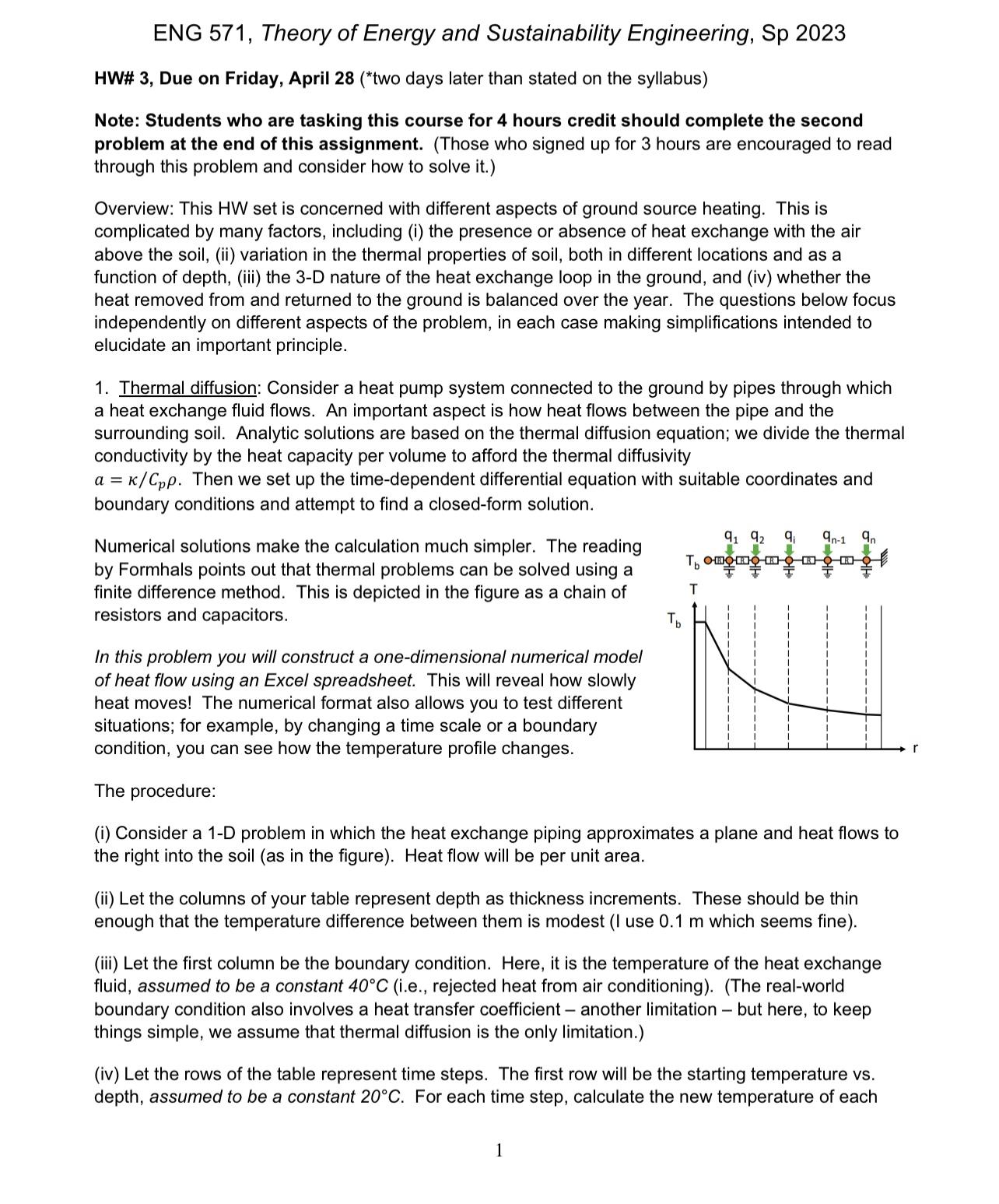
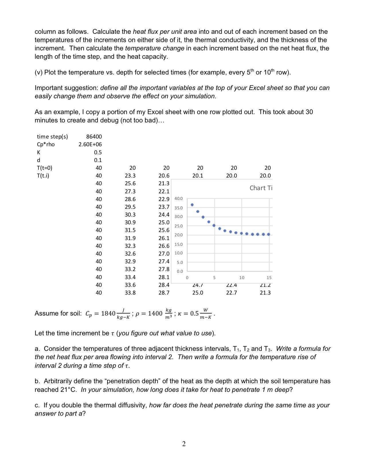
ENG 571, Theory of Energy and Sustainability Engineering, Sp 2023 HW# 3, Due on Friday, April 28 (*two days later than stated on the syllabus) Note: Students who are tasking this course for 4 hours credit should complete the second problem at the end of this assignment. (Those who signed up for 3 hours are encouraged to read through this problem and consider how to solve it.) Overview: This HW set is concerned with different aspects of ground source heating. This is complicated by many factors, including (i) the presence or absence of heat exchange with the air above the soil, (ii) variation in the thermal properties of soil, both in different locations and as a function of depth, (iii) the 3-D nature of the heat exchange loop in the ground, and (iv) whether the heat removed from and returned to the ground is balanced over the year. The questions below focus independently on different aspects of the problem, in each case making simplifications intended to elucidate an important principle. 1. Thermal diffusion: Consider a heat pump system connected to the ground by pipes through which a heat exchange fluid flows. An important aspect is how heat flows between the pipe and the surrounding soil. Analytic solutions are based on the thermal diffusion equation; we divide the thermal conductivity by the heat capacity per volume to afford the thermal diffusivity a = /Cpp. Then we set up the time-dependent differential equation with suitable coordinates and boundary conditions and attempt to find a closed-form solution. Numerical solutions make the calculation much simpler. The reading by Formhals points out that thermal problems can be solved using a finite difference method. This is depicted in the figure as a chain of resistors and capacitors. In this problem you will construct a one-dimensional numerical model of heat flow using an Excel spreadsheet. This will reveal how slowly heat moves! The numerical format also allows you to test different situations; for example, by changing a time scale or a boundary condition, you can see how the temperature profile changes. The procedure: T 91 92 9. qn-1 9n (i) Consider a 1-D problem in which the heat exchange piping approximates a plane and heat flows to the right into the soil (as in the figure). Heat flow will be per unit area. (ii) Let the columns of your table represent depth as thickness increments. These should be thin enough that the temperature difference between them is modest (I use 0.1 m which seems fine). (iii) Let the first column be the boundary condition. Here, it is the temperature of the heat exchange fluid, assumed to be a constant 40C (i.e., rejected heat from air conditioning). (The real-world boundary condition also involves a heat transfer coefficient - another limitation - but here, to keep things simple, we assume that thermal diffusion is the only limitation.) (iv) Let the rows of the table represent time steps. The first row will be the starting temperature vs. depth, assumed to be a constant 20C. For each time step, calculate the new temperature of each 1 column as follows. Calculate the heat flux per unit area into and out of each increment based on the temperatures of the increments on either side of it, the thermal conductivity, and the thickness of the increment. Then calculate the temperature change in each increment based on the net heat flux, the length of the time step, and the heat capacity. (v) Plot the temperature vs. depth for selected times (for example, every 5th or 10th row). Important suggestion: define all the important variables at the top of your Excel sheet so that you can easily change them and observe the effect on your simulation. As an example, I copy a portion of my Excel sheet with one row plotted out. This took about 30 minutes to create and debug (not too bad)... time step(s) 86400 Cp*rho 2.60E+06 K 0.5 d 0.1 T(t=0) 40 20 20 1 T(t.i) 40 23.3 20.6 | 40 25.6 21.3 20 20.1 20 20 20.0 20.0 Chart Ti 40 27.3 22.1 40 28.6 22.9 40.0 40 29.5 23.7 35.0 40 30.3 24.4 30.0 40 30.9 25.0 25.0 40 31.5 25.6 20.0 40 31.9 26.1 40 32.3 26.6 15.0 40 32.6 27.0 10.0 40 32.9 27.4 5.0 40 33.2 27.8 0.0 40 33.4 28.1 0 5 10 15 40 33.6 28.4 40 33.8 28.7 24.7 25.0 22.4 21.2 22.7 21.3 Assume for soil: Cp = 1840 kg kg-K ; p = 1400 W ; K = 0.5 m3 m-K Let the time increment be (you figure out what value to use). a. Consider the temperatures of three adjacent thickness intervals, T1, T2 and T3. Write a formula for the net heat flux per area flowing into interval 2. Then write a formula for the temperature rise of interval 2 during a time step of t. b. Arbitrarily define the "penetration depth" of the heat as the depth at which the soil temperature has reached 21C. In your simulation, how long does it take for heat to penetrate 1 m deep? c. If you double the thermal diffusivity, how far does the heat penetrate during the same time as your answer to part a? 2 d. How does the heat flow from the heat exchange fluid (the boundary condition) into the first thickness increment change over time? You can create a new column with that information. e. In order to maintain a constant heat flow from the heat exchange fluid into the first thickness increment at all times, how should the temperature in the fluid change? Give a short explanation. To gain further insight (but nothing to turn in), play with this simulation. For example, as the starting condition you can insert a higher temperature in just one increment in the middle of the sample and watch it spread in time. ==> The following problem is only for students who signed up for four hours credit. 2. Cylindrical bore hole field: In a conventional geothermal installation, the heat transfer fluid is delivered in parallel to all the boreholes (an example is the Campus Instructional Facility). The soil in between all the boreholes warms up or cools down in the same manner, which involves diffusion of heat into the soil between neighboring bore holes. By contrast, the ESTCP video (https://www.youtube.com/watch?v=-hSLP4JpPvU) shows an arrangement in which the heat transfer fluid flows in series from the center towards the outside, or vice-versa. That intentionally creates a temperature gradient in the soil between the center and outside of the bore hole field. The direction of fluid flow is reversed between seasons. Here, the bore hole field is so large that, as an approximation, we do NOT need to consider thermal diffusion in the soil. Instead, the soil warms up or cools down only by exchanging heat with the heat transfer fluid. This approximation is justified by the answer to problem 1. To model this situation in the simplest possible way, we neglect the cylindrical geometry of the ESTCP bore hole field and assume it is a long straight pipe in which the heat exchange fluid flows, surrounded by a cylindrical volume of soil. The key point is that temperature of both the fluid and the surrounding soil will vary along the length of the structure. Fluid flows through a pipe of inner radius r at a flow rate Q [m/sec]. The surrounding soil has a radius R. Assume that heat can flow from fluid to soil according to Q = U AT, where U is a heat transfer coefficient [W/m K] at the wall of the pipe and AT is the temperature difference between fluid and surrounding soil. (Sorry about the use of both Q and Q...I am keeping with usual notation.) a. For an incremental length dl of pipe, what is the heat flux for a temperature difference of AT? (This does not involve the flow of the fluid.) b. The fluid has a heat capacity of Cf [J/m K]. In a time interval dt, what is the temperature change dT of the fluid in the increment dl? c. For a flow rate Q, what is the average fluid velocity dl/dt along the pipe? d. Given your answers to a.-c., what is the gradient in fluid temperature dT/dl as it flows along the pipe? Your expression should contain AT, U, Cf, r and Q. Note that in your answer, you have two independent ways to change the temperature gradient! 3 e. In summer, a heat pump air conditioner adds heat to the soil. Assume that in a conventional parallel installation, all the soil is heated uniformly to 30C. By contrast, in a series installation, the same amount of heat raises the temperature to 40C on one end but, due to the cooling of the heat transfer fluid as it flows along the pipe, the temperature remains at 20C at the other end. In the following winter, what is the maximum fluid temperature that can be extracted from the soil in the parallel installation? in the series installation? f. The ESTCP video notes that in winter, the fluid is cooled by passing through an outside air heat exchanger prior to passing through the borehole field in order to be warmed up! This appears to make no sense. But why is it done? Give a short answer. Hint: the total heat rejection by air conditioning in the summer is larger than the total heat extraction for heating in the winter. This problem reveals the possible utility of counter-flow heat exchange. In the full optimization problem, we need to calculate the total efficiency (or exergy loss) in each case, considering the required fluid temperature to reject or extract heat from the ground. Not simple, but fun! 4